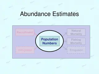
Understanding Capture-Mark-Recapture Models for Closed Populations

Utilize the MARK software program to analyze capture-recapture data on rabbit populations. Learn how to set up parameters, run models, and estimate population abundance using multi-sample capture-mark-recapture techniques. Explore the data, define parameter structures, and interpret model outputs to gain insights into population dynamics.

Download Presentation

Please find below an Image/Link to download the presentation.
The content on the website is provided AS IS for your information and personal use only. It may not be sold, licensed, or shared on other websites without obtaining consent from the author. Download presentation by click this link. If you encounter any issues during the download, it is possible that the publisher has removed the file from their server.
E N D
Presentation Transcript
Introduction to Capture-Mark-Recapture Lab 5 Closed Population Models
Install program MARK Free software program for doing capture -mark- recapture Served out of CSU, maintained by Gary White and Evan Cooch Google Program MARK http://www.phidot.org/software/mark/downloads/
Install RMark This is our link to run MARK from R. So install RMarkand then attach the library install.packages( RMark ) library(RMark) #Removes all objects stored in your workspace rm(list = ls())
Multi-sample CMR in RMark A capture-recapture data set on rabbits: Edwards, W.R. and L.L. Eberhardt 1967. Estimating cottontail abundance from live trapping data. J. Wildl. Manage. 31:87-96. ###read in data set ### data(edwards.eberhardt) ## assign the dataset a convenient name ### dat<-edwards.eberhardt
Looking at the data ###examine the data head(dat) ch 1 000000000000000001 2 000000000000000001 3 000000000000001000 4 000000000000001000 5 000000000000001000 6 000000000000001000 # ch = capture history # what do you notice about the data?
Set up the parameters #step 1: define parameter structure #the first element defines covariates on detection #the second element defines if p and c are the same p0<-list(formula = ~1, share = TRUE) #structure for model M0 pt<-list(formula=~time, share = TRUE) #structure for model Mt pb<-list(formula=~1, share = FALSE) #structure for model Mb
Run Model M0 #model m0 -no variation in detection m0<-mark(data=dat, model = "Closed", model.parameters = list(p = p0) ) summary(m0)
> summary(m0) Output summary for Closed model Name : p(~1)c()f0(~1) Npar: 2 -2lnL: 375.5941 AICc: 379.6029 Beta estimate se lcl ucl p:(Intercept) -2.416076 0.1171742 -2.645738 -2.186414 f0:(Intercept) 3.008588 0.3395372 2.343095 3.674081 Real Parameter p 1 2 3 4 5 6 7 8 0.081955 0.081955 0.081955 0.081955 0.081955 0.081955 0.081955 0.081955 . Real Parameter c 2 3 4 5 6 7 8 9 0.081955 0.081955 0.081955 0.081955 0.081955 0.081955 0.081955 0.081955 . Add fo to the number captured (here, 76) to get the estimate of abundance = 96.258 Real Parameter f0 1 20.25877
Looking at the MARK output Estimates of Derived Parameters Population Estimates of { p(~1)c()f0(~1) } 95% Confidence Interval Grp. Sess. N-hat Standard Error Lower Upper ---- ----- -------------- -------------- -------------- -------------- 1 1 96.258775 6.8786049 86.603282 114.70669
Model Mt # model mt : p=c, but p varies with time #previously set up the function for the detection: #pt<- list(formula=~time, share = TRUE) #structure for model Mt mt<- mark(data=dat, model="Closed", model.parameters = list(p=pt))
Model Mb #model mb - p does not equal c #pb<-list(formula=~1, share = FALSE) #structure for model Mb mb<-mark(data=dat, model ="Closed", model.parameters = list(p=pb))
Model selection by AIC #automatically collects all models; mlist<-collect.models() #creates a table with model results, sorted by AIC model.table(mlist) NOTE: When comparing models with AIC using Rmark, it is important that you check the number of parameters and that you are only comparing models that are all analyzed with the same likelihood (full vs. conditional).
Model Selection Table model npar AICc DeltaAICc weight Deviance 4 p(~time)c()f0(~1) 19 354.5968 0.00000 9.384175e-01 305.2648 5 p(~time)c(~1)f0(~1) 20 360.0446 5.44779 6.157771e-02 308.6528 1 p(~1)c()f0(~1) 2 379.6029 25.00616 3.486397e-06 364.8259 2 p(~1)c(~1)f0(~1) 3 381.5498 26.95302 1.317112e-06 364.7640
Now onto the lab activity Note: when you want to read in your own data from a text file, you must read the data into R using the following: dat<-import.chdata( datafile.txt", header=T) This will make your text file in the proper format for Mark to use.


")