Understanding Sampling Distributions and Central Limit Theorem in Statistics

This content covers various topics such as mean diameter of cherries, sampling distributions, random variables, and the central limit theorem. It explains concepts with examples like throwing dice, calculating sample means, and exploring the distribution of random variables. The content delves into how repeated sampling can help estimate population parameters and understand the variability of sample means.

Download Presentation

Please find below an Image/Link to download the presentation.
The content on the website is provided AS IS for your information and personal use only. It may not be sold, licensed, or shared on other websites without obtaining consent from the author. Download presentation by click this link. If you encounter any issues during the download, it is possible that the publisher has removed the file from their server.
E N D
Presentation Transcript
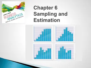
Chapters 1. Introduction 2. Graphs 3. Descriptive statistics 4. Basic probability 5. Discrete distributions 6. Continuous distributions 7. Central limit theorem 8. Estimation 9. Hypothesis testing 10. Two-sample tests 13. Linear regression 14. Multivariate regression Chapter 7 Sampling Distribution and Central Limit Theorem
What is the Mean Diameter of a Cherry 1. Take a sample, measure their diameters and get the mean. What do we have? Is it the mean diameter of the population? Is it close to the population mean? 2. Take another sample with same sample size get the sample mean. Do we have anything new? Is it the same as the first? Is it the population mean? Is it close to? 3. Take sample after sample, with the same sample size, calculate mean after mean. What do we have? Data for the sample mean. 10/5/2024 Towson University - J. Jung 9.2
Another Thought Suppose 3 cherries are drawn and diameters are measured. We have three observations of a random variable, each of which comes from the same distribution. Call them d1, d2 and d3. Sample mean is X=1/3*d1+1/3*d2+1/3*d3 Linear Combination of R.V.s ! X-bar is R.V., too! X-bar has its own distribution, called Sampling Distribution of the mean. Then we can work out the mean and standard error (the standard deviation of the sampling distribution) for X-bar using formula from linear combination. 10/5/2024 Towson University - J. Jung 9.3
1 Sampling Distribution of averages Throw a fair die, Random variable X = # of spots on any throw. The probability distribution of X is: x 1 2 3 4 5 6 P(x) 1/6 1/6 1/6 1/6 1/6 1/6 and the mean and variance are calculated as well: 10/5/2024 Towson University - J. Jung 9.4
Throw a Die Two Times 36 possible samples of size 2, only 11 values, and some occur more frequently than others. 10/5/2024 Towson University - J. Jung 9.5
Sampling Distribution of Two Dice The sampling distribution of is shown below: 6/36 P( ) 5/36 1.0 1.5 2.0 2.5 3.0 3.5 4.0 4.5 5.0 5.5 6.0 1/36 2/36 3/36 4/36 5/36 6/36 5/36 4/36 3/36 2/36 1/36 4/36 P( ) 3/36 2/36 1/36 1.0 1.5 2.0 2.5 3.0 3.5 4.0 4.5 5.0 5.5 6.0 10/5/2024 Towson University - J. Jung 9.6
Compare Compare the distribution of X 1.0 1.5 2.0 2.5 3.0 3.5 4.0 4.5 5.0 5.5 6.0 1 2 3 4 5 6 with the sampling distribution of . As well, note that: 10/5/2024 Towson University - J. Jung 9.7
Generalize We can generalize the mean and variance of the sampling of two dice: to n-dice: The standard deviation of the sampling distribution is called the standard error: 10/5/2024 Towson University - J. Jung 9.8
Central Limit Theorem The sampling distribution of the mean of a random sample drawn from any population is approximately normal for a sufficiently large sample size. The larger the sample size, the more closely the sampling distribution of X-bar will resemble a normal distribution. In many practical situations, a sample size of 30 may be sufficiently large. However, if the population is normal, then X-bar is exactly normal for all values of n. 10/5/2024 Towson University - J. Jung 9.9
Sampling Distribution of the Sample Mean 1. 2. 3. If X is normal, X is normal. If X is non-normal, X is approximately normal for sufficiently large sample sizes. Note: the definition of sufficiently large depends on the extent of non-normality of x (e.g. heavily skewed; multimodal) Approximations become good once n 30. 10/5/2024 Towson University - J. Jung 9.10
Central Limit Theorem 10/5/2024 Towson University - J. Jung 9.11
Central Limit Theorem 10/5/2024 Towson University - J. Jung 9.12
Example The foreman of a bottling plant has observed that the amount of soda in each 32-ounce bottle is actually a normally distributed random variable, with a mean of 32.2 ounces and a standard deviation of 0.3 ounce. If a customer buys one bottle, what is the probability that the bottle will contain more than 32 ounces? If a customer buys a carton of four bottles, and measure the mean amount of the four bottles . Will it be 32.2? Suppose the customer gets a mean of 32, is it the population mean? What is the probability that the mean amount of the four bottles will be greater than 32 ounces? 10/5/2024 Towson University - J. Jung 9.13
Example We want to find P(X > 32), where X is normally distributed with =32.2 and =.3 1) X is normally distributed, therefore so will X. Things we know: 2) = 32.2 oz. 3) 10/5/2024 Towson University - J. Jung 9.14
Graphically Speaking mean=32.2 what is the probability that one bottle will contain more than 32 ounces? what is the probability that the mean of four bottles will exceed 32 oz? 10/5/2024 Towson University - J. Jung 9.15
Standardizing the Sample Mean The sampling distribution can be used to make inferences about population parameters. In order to do so, the sample mean can be standardized to the standard normal distribution using the following formulation: 10/5/2024 Towson University - J. Jung 9.16
Sampling Distribution of a Proportion The estimator of a population proportion of successes is the sample proportion. That is, we count the number of successes in a sample and compute: p = X n X is the number of successes, n is the sample size. P can be any value between 0 and 1, so is continuous variable. Enable us to transform categorical variables into quantitative variables. P is the sample version of , just like X-bar is the sample version of When and 5 n 1 ( n n 10/5/2024 Towson University - J. Jung ) 5 1 ( ) ~ , p N 9.17
Example: Sample Proportions Suppose the proportion of voters that support the Democratic party in the US is 52%. 1. Randomly select a voter. What is the probability that a Democrat is selected? 2. What is the probability of selecting a sample of 100 voters, in which the proportion of Democrats is: Equal to 55% Less than 50% Between 40% and 52% 10/5/2024 Towson University - J. Jung 9.18
Answers 1. Since proportion of Dems is 52%, the chance to pick a Democrat in a random draw is 52%. 2. Can proportion be assumed normally distributed?: 1. 0.52*100 = 52 >= 5 2. 0.48*100 = 48 >= 5 Then p ~ N(0.52, sqrt((0.52*0.48) / 100)) P(p=55%) = 0 P(p<=50%) = NORM.S.DIST((0.50-0.52)/ 0.04996,1) P(40%<=p<=52%) = NORM.S.DIST((0.52-0.52)/0.04996,1) NORM.S.DIST((0.40-0.52)/0.04996,1) 10/5/2024 Towson University - J. Jung 9.19
Summary CLT: sample averages Population Sample 1: n = 60 ?1 ? is a random variable By the CLT, it follows a normal distribution: Sample 2: n = 60 Random variable X has unknown distribution: ?2 . ?~? ?,? ?~?(?,?) ? Sample 100: n = 60 if n>30 ?100 10/5/2024 Towson University - J. Jung 9.20
Summary CLT: sample proportions Population Sample 1: n = 60 ?1 ? is a random variable By the CLT, it follows a normal distribution: Sample 2: n = 60 True population proportion : ?2 ? . ?(1 ?) ? ?~? ?, Sample 100: n = 60 if: n ? 5 n (1 ?) 5 ?100 10/5/2024 Towson University - J. Jung 9.21