Understanding Linear Regression Models and Terminology

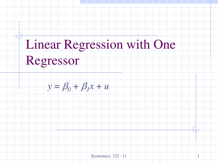
Linear Regression with One Regressor y = 0 + 1x + u Economics: 332 - 11 1

Outline 1. The population linear regression model 2. The ordinary least squares (OLS) estimator and the sample regression line 3. Measures of fit of the sample regression 4. The least squares assumptions 5. The sampling distribution of the OLS estimator 2

The Linear Regression Model Establish a causal relationship: Test Score = 0 + 1Number of handouts 1 = slope of population regression line = Handouts Test score = change in test score for a unit change in Handouts Why are 0 and 1 population parameters? We would like to know the population value of 1. We don t know 1, so must estimate it using data. 3

The Linear Regression Model Regression allows us to estimate the slope of the population regression line. The slope of the population regression line is the expected effect on Y of a unit change in X. Ultimately our aim is to estimate the causal effect on Y of a unit change in X. 4

Some Terminology Regression analysis with cross-sectional data Purpose: Explaining the relationship between Y and X variables with a model (Explain a variable Y in terms of Xs) In the simple linear regression model, where y = 0 + 1x + u, we typically refer to y as the Dependent Variable, or Left-Hand Side Variable, or Explained Variable 5

Some Terminology, cont. In the simple linear regression of y on x, we typically refer to x as the Independent Variable, or Right-Hand Side Variable, or Explanatory Variable, or Regressor, or Covariate, or Control Variables 6

Some Terminology, cont. The variable u called the error term and represents factors other than x that affect y. Factors that we cannot observe: motivation 0 and 1 : parameters to estimate. 7

Error term Error exists because Other important variables might be omitted Measurement error 1. 2. Understand error structure and minimize error

A Simple Assumption If the other factors in u held fixed, so that the change in u is zero, u = 0. The average value of u, the error term, in the population is 0. That is, E(u) = 0: simply makes a statement about the distribution of the unobservables in the population. 9

Zero Conditional Mean We are only able to get reliable estimators of 0 and 1 from a random sample of data when we make an assumption restricting how the unobservable u is related to the explanatory variable x. Without such a restriction, we will not be able to estimate the ceteris paribus effect, 1. 10

Zero Conditional Mean We need to make a crucial assumption about how u and x are related We want it to be the case that knowing something about x does not give us any information about u, so that they are completely unrelated. That is, that E(u|x) = E(u) = 0, which implies E(y|x) = 0 + 1x 11

Zero Conditional Mean The crucial assumption is that the average value of u does not depend on the value of x. E(u|x) = E(u) = 0 : says that, for any given value of x, the average of the unobservables is the same and therefore must equal the average value of u in the population. 12

Zero Conditional Mean E(y|x) = 0 + 1x E(y|x), is a linear function of x. The linearity means that a one-unit increase in x changes the expected value of y by the amount 1. 13

Example A model relating a person s wage to observed education and other unobserved factors. If wage is measured in dollars per hour and educ is years of education Then 1 measures the change in hourly wage given another year of education, holding all other factors fixed. Some of those factors include innate ability, work ethic, and innumerable other things. 14

Ordinary Least Squares Basic idea of regression is to estimate the population parameters from a sample Let {(xi,yi): i=1, ,n} denote a random sample of size n from the population i is an index. If we are analyzing people, then this typically refers to the person For each observation in this sample, it will be the case that yi = 0 + 1xi + ui 15

Covariate, RHS variable, Predictor, independent variable Intercept Error Term Dependent variable Outcome measure 16

Estimator A statistic 1 that provides information on the parameter of interest (e.g., consumption) Generated by applying a function to the data

Population regression line and the associated error terms E(y|x) = 0 + 1x y . y4 { u4 . u3 y3 } . y2 u2 { u1 . } y1 x2 x1 x4 x3 x 18

Deriving OLS Estimates How can we estimate 0and 1 from data? To derive the OLS estimates we need to realize that our main assumption of E(u|x) = E(u) = 0 also implies that Cov(x,u) = E(xu) = 0 Why? Remember from basic probability that Cov(X,Y) = E(XY) E(X)E(Y) 19

Deriving OLS continued We can write our 2 restrictions (E(u) = 0, E(xu) = 0) just in terms of x, y, 0 and , since u = y 0 1x E(y 0 1x) = 0 E[x(y 0 1x)] = 0 This implies two restrictions on the joint probability distribution of (x,y) in the population. 20

More Derivation of OLS The sample versions are as follows: ( ) n = n = 1 0 n y x 0 1 i i 1 i ( ) = i = 1 0 n x y x 0 1 i i i 1 21

More Derivation of OLS Given the definition of a sample mean, and properties of summation, we can rewrite the first condition as follows = + , y or x 0 1 = y x 0 1 22

More Derivation of OLS ( ( ) ) n = i = 0 x y y x x 1 1 i i i 1 n n ( ) ( ) = i = i = x y y x x x 1 i i i i 1 1 n n ( )( ) ( ) = i = i 2 = x x y y x x 1 i i i 1 1 23

So the OLS estimated slope is n ( )( ) = i x x y y i i = 1 1 n ( ) = i 2 x x i 1 n ( ) = i 2 provided that 0 x x i 1 24

OLS: Predicted value and residual - Once we have determined the OLS intercept and slope estimates, we form the OLS regression line: - The notation y , read as y hat, denotes that the predicted values are estimates. - There is a predicted value for each observation in the sample. - The intercept, 0, is the predicted value of y when x = 0. - The residual for observation i is : 25

Summary of OLS slope estimate The slope estimate is the sample covariance between x and y divided by the sample variance of x If x and y are positively correlated, the slope will be positive If x and y are negatively correlated, the slope will be negative 26

More on OLS Intuitively, OLS is fitting a line through the sample points such that the sum of squared residuals (error term) is as small as possible, hence the term least squares The residual, , is an estimate of the error term, u, and is the difference between the fitted line (sample regression function) and the sample point: 27

Sample regression line, sample data points and the associated estimated error terms y . y4 { 4 = + y x 0 1 . 3 y3 } . y2 2 { 1 . } y1 x2 x1 x4 x3 x 28

Population regression line and sample regression line 29

A Note on Terminology We will often indicate that an equation has been obtained by OLS in saying that we run the regression ofy on x. or simply that we regress y on x. The positions of y and x indicate which is the dependent variable and which is the independent variable: we always regress the dependent variable on the independent variable. 30

A Real Causal Model We will think about our model (i.e. y = 0 + 1x + u) in this way: 1and 0are real numbers which are not known and we want to uncover them We choose X Nature chooses U in a way that is unrelated to our choice of X 31

Return to Education Example If the model is indeed y = 0 + 1x + u, and u is unrelated to your college going decision (x)... u it kind of doesn t really matter Actually, It is thing that affect your earnings (y) other than education. Examples: Intelligence, Family Connections, Motivation, etc. 32

Return to Education Example let y = wage, where wage is measured in dollars per hour for a particular person, if wage = 6.75, the hourly wage is $6.75 Let x = educ denote years of schooling; for example, educ = 12 corresponds to a complete high school education 33

Return to Education Example Interpretation of the Estimates Using the data, where n = 526 individuals, we obtain the following OLS: The intercept of 0.90 literally means that a person with no education has a predicted hourly wage of 90 cents an hour. 34

Return to Education Example For a person with eight years of education, the predicted wage is wage^ = 0.90 + 0.54(8) = 3.42, or $3.42 per hour. The slope estimate implies that one more year of education increases hourly wage by 54 cents an hour. Therefore, four more years of education increase the predicted wage by 4(0.54) = 2.16, or $2.16 per hour. 35

Voting Outcomes and Campaign Expenditures Let voteA be the percentage of the vote received by Candidate A shareA: is the percentage of total campaign expenditures accounted for by Candidate A. We can estimate a simple regression model to find out whether spending more implies a higher percentage of the vote. 36

Voting Outcomes and Campaign Expenditures The estimated equation using the 173 observations is: This means that if the share of Candidate A s spending increases by one percentage point, Candidate A receives almost one-half a percentage point (0.464) more of the total vote. 37

OLS regression: STATA output F( 1, 418) = 19.26 Prob > F = 0.0000 R-squared = 0.0512 Root MSE = 18.581 ------------------------------------------------------------------------- | Robust Y | Coef. Std. Err. t P>|t| [95% Conf. Interval] --------+---------------------------------------------------------------- X | -2.279808 .5194892 -4.39 0.000 -3.300945 -1.258671 _cons | 698.933 10.36436 67.44 0.000 678.5602 719.3057 ------------------------------------------------------------------------- regress testscr str, robust Regression with robust standard errors Number of obs = 420 (We ll discuss the rest of this output later.)