Linear Regression and Classification Methods


Linear Regression and Classification

Outline
I. Line fitting and gradient descent
II. Multivariable linear regression
III. Linear classifiers
IV. Logistic regression

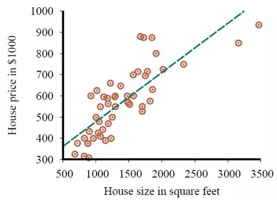
I. Linear Regression

Hypothesis space: univariate linear functions.


inputs
outputs

Houses for sale in Berkeley, CA
Line Fitting
Vanishing of Partial Derivatives
Plot of the Loss Function
Convex function with n
o local minima.
Gradient Descent
Compute an estimate of the gradient of the loss function.
Move a small amount in the direction of the negative gradient, i.e.,
the steepest downhill direction.
Repeat until convergence on a point with (local)
minimum loss.
step size or
learning rate
Instead, the method of gradient descent is used:
** To see how gradient descent works, see Section 4 of
https://faculty.sites.iastate.edu/jia/files/inline-files/nonlinear-program.pdf
.
Multivariable Linear Regression
Hypothesis space:
Best weight vector:
Optimal Weights
Regularization
Commonly applied on multivariable linear function to avoid overfitting.
where
III. Linear Classifiers
Same domain with more data points.
earthquakes
nuclear
explosions
Linear Separator
A
decision boundary
is a line that
separates two classes.
A
linear separator
is a linear decision
boundary.
Classification hypothesis
:
Not linearly
separable!
Learning Rule
Use the
perceptron learning rule
(essentially borrowed from gradient descent):
Training Curves for Perceptron Learning
The learning rule is applied one example at a time.
A
training curve
measures the classifier performance on a fixed
training set
as learning proceeds one example at a time on the same set.
657 steps before convergence
63 examples, each used 10 times on average
Training Curves (cont’d)
Fails to converge after 10,000 steps.
Data not linearly separable.
IV. Logistic Function
Current hypothesis function is not continuous, let alone differentiable.
This makes learning with the perceptron rule
very unpredictable.
It would be better if some examples could be classified as unclear
borderline cases.
Use a continuous, differential function to soften the threshold
Logistic function
:
Hypothesis function:
Logistic Regression
Still apply gradient descent.
Weight update:
Improvements on Training Results
Logistic regression converges
far more quickly and reliably.
Explore the concepts of line fitting, gradient descent, multivariable linear regression, linear classifiers, and logistic regression in the context of machine learning. Dive into the process of finding the best-fitting line, minimizing empirical loss, vanishing of partial derivatives, and utilizing gradient descent for optimization. Discover how these methods are applied in modeling data points and making predictions in various scenarios.

Uploaded on Sep 18, 2024 | 0 Views
Download Presentation

Please find below an Image/Link to download the presentation.
The content on the website is provided AS IS for your information and personal use only. It may not be sold, licensed, or shared on other websites without obtaining consent from the author.If you encounter any issues during the download, it is possible that the publisher has removed the file from their server.
You are allowed to download the files provided on this website for personal or commercial use, subject to the condition that they are used lawfully. All files are the property of their respective owners.
The content on the website is provided AS IS for your information and personal use only. It may not be sold, licensed, or shared on other websites without obtaining consent from the author.
E N D
Presentation Transcript
Linear Regression and Classification Outline I. Line fitting and gradient descent II. Multivariable linear regression III. Linear classifiers IV. Logistic regression * Figures are from the textbook site.
I. Linear Regression Data points: ?1,?1, ?2,?2, , ??,?? inputs outputs Houses for sale in Berkeley, CA Hypothesis space: univariate linear functions. ?(?) ?1? + ?0 (?0,?1) Linear regression: Find the ? that best fits the data.
Line Fitting We find the weights (?0,?1) that minimizes the empirical loss. Use the squared-error loss ?2?, ? = ? ? 2, summed over all the points. ? Loss ? = ?2(??, ?(??)) ?=1 ? 2 = ?? ?(??) ?=1 ? 2 = ?? (?1??+ ?0) ?=1 ? = argmin Loss ? ?
Vanishing of Partial Derivatives At the minimizing ?, the gradient of Loss ? must vanish: ?Loss ??0 ,?Loss ??1 ? = 0.232? + 246 Loss ? = = 0 ? ?Loss ??0 ? 2= 0 = ??0 ?? (?1??+ ?0) ?=1 ? ?Loss ??1 ? 2= 0 = ??1 ?? (?1??+ ?0) ?=1 Note: the best-fit line does not minimize the sum of squares of distances of the data points to the line. The model ?(?) ?1? + ?0 is inferior to the general line equation ?? + ?? + ? = 0, which is used in computer vision for the purpose of extracting straight edges from an image. The reason is that ?(?) ?1? + ?0 cannot represent a vertical line so the fitting result becomes undesirable when the slope gets very large. ? ? ? ?1=? ?=1 ???? ?=1 ?? ?=1 ?? 2 ? 2 ?=1 ? ? ?=1 ?? ?? ? ? ?0=1 ?? ?1 ?? ? ?=1 ?=1
Plot of the Loss Function ? 2 Loss ? = ?? (?1??+ ?0) ?=1 Convex function with no local minima.
Gradient Descent For a complex loss function, vanishing of its gradient often results in a system of nonlinear equations in ? that does not have a closed-form solution. Instead, the method of gradient descent is used: Start at a point ? in the weight space. Compute an estimate of the gradient of the loss function. Move a small amount in the direction of the negative gradient, i.e., the steepest downhill direction. Repeat until convergence on a point with (local) minimum loss. ? any point in the parameter space while not converged do for each ?? in ?do ?? ?? ? ? ?,? = cos2? + cos2?2 ? ???Loss(?) Gradient map step size or learning rate * Section 19.6.2 applies gradient descent to a quadratic loss function, which defeats the purpose since the gradient Loss ? is linear in ? whose values can be easily determined from solving the linear system Loss ? = 0. ** To see how gradient descent works, see Section 4 of https://faculty.sites.iastate.edu/jia/files/inline-files/nonlinear-program.pdf.
Multivariable Linear Regression An example is represented by an ?-vector ??= (??,1, ,??,?). Hypothesis space: ? ?? = ?0+ ?1?1+ + ????= ?0+ ???? ?=1 For convenience, we extend ? by adding ?0= 1 such that ? = (1,?1, ,??). ?? = ? ? Best weight vector: ? = argmin ?2(??,? ??) ? ?
Optimal Weights Write ? as a column vector, i.e., ? = ?0,?1, ,?? Vector of ? outputs: ? = ?1,?2, ,?? ?. ?. ?1 ?? Data matrix (? ?): ? = Predicted outputs: ? = ?? Loss over all the training data: ? ? = ? ? 2= ?? ? 2 0 = ? ? = ?? ???? ? ???? ??? = 0 ? almost always has full rank since ? ? 1??? ? = ? = ??? pseudoinverse of ?
Regularization Commonly applied on multivariable linear function to avoid overfitting. Cost( ?)= EmpLoss ? + ?Complexity( ?) where ? |??|? Complexity ? = ??? = ?=1 ?1 (with ? = 1) regularization tends to produce a sparse model (in which many weights are set to zero) because it takes the ?0,?1, ,?? axes seriously. ?2 (with ? = 2) regularization takes the dimension axes arbitrarily.
III. Linear Classifiers earthquakes nuclear explosions Seismic data for earthquakes and nuclear explosions: ?1 and ?2 respectively refer to body and surface wave magnitudes computed from the seismic signal. Same domain with more data points. Task Learn a hypothesis that will take new (?1,?2) points and return 0 for earthquakes and 1 for explosions.
Linear Separator A decision boundary is a line that separates two classes. A linear separator is a linear decision boundary. e.g., 4.9 + 1.7?1 ?2= 0 ? = ?0,?1, ,?? ? = ?0,?1, ,?? ? = 1 Classification hypothesis: Not linearly separable! 1 if ?? 0 ?(?) = 0 if ?? < 0
Learning Rule 1 if ?? 0 Gradient ? either vanishes or is undefined. ?(?) = 0 if ?? < 0 Use the perceptron learning rule (essentially borrowed from gradient descent): ?? ??+ ?(?? ?(??))??,? on a single example (??,?) ??= ?(??). The output is correct, so no change of weights. ??= 1 but ??? = 0. ??is increased if ??,?> 0 and decreased if ??,?< 0. In both situations, ?? increases with the intention to output 1. ??= 0 but ??? = 1. ??is decreased if ??,?> 0 and increased if ??,?< 0. In both situations, ?? decreases with the intention to output 0.
Training Curves for Perceptron Learning The learning rule is applied one example at a time. A training curve measures the classifier performance on a fixed training set as learning proceeds one example at a time on the same set. ? = 1 657 steps before convergence 63 examples, each used 10 times on average
Training Curves (contd) Data not linearly separable. Fails to converge after 10,000 steps. Let ? decay as ?(1/?) where ? = # iterations. ?? ??+ ?(?? ?(??))??,? e.g., ? ? = 1000/(1000 + ?)
IV. Logistic Function Current hypothesis function is not continuous, let alone differentiable. This makes learning with the perceptron rule very unpredictable. It would be better if some examples could be classified as unclear borderline cases. Use a continuous, differential function to soften the threshold Hypothesis function: Logistic function: 1 1 Logistics ? = ?(?) = ?? = Logistics ?? = 1+? ? 1 + ? ?? 1 if ?? 0 ?(?) = 0 if ?? < 0
Logistic Regression Fit the model ?? = Logistics ?? to minimize loss on a data set. Still apply gradient descent. 1 Logistics ? = ?(?) = 1 + ? ? ? ? 2 Loss ? = ? ?? ??? ??? = 2(? ?? ) ? (??) ?? ? ?? = ?(??)(1 ? ?? ) = ?? (1 ?? ) = 2(? ?? ) ?? (1 ?? ) ?? Weight update: ?? ??+ ?(? ?? ) ?? (1 ?? ) ??
Improvements on Training Results ? ? = 1000/(1000 + ?) Logistic regression converges far more quickly and reliably. ? ? = 1000/(1000 + ?) ? = 1 ? = 1


")