Methods for Handling Collinearity in Linear Regression

Linear regression can face issues such as overfitting, poor generalizability, and collinearity when dealing with multiple predictors. Collinearity, where predictors are linearly related, can lead to unstable model estimates. To address this, penalized regression methods like Ridge and Elastic Net can be used, as well as approaches like Principal Components Regression (PCR) and Partial Least Squares Regression (PLSR). These methods help mitigate collinearity and improve model performance in situations with many predictors.

• Linear Regression
• Collinearity
• Penalized Regression
• PCR
• PLSR

mklas Follow

Uploaded on Sep 18, 2024 | 1 Views

Download Presentation

Please find below an Image/Link to download the presentation.

The content on the website is provided AS IS for your information and personal use only. It may not be sold, licensed, or shared on other websites without obtaining consent from the author.If you encounter any issues during the download, it is possible that the publisher has removed the file from their server.

You are allowed to download the files provided on this website for personal or commercial use, subject to the condition that they are used lawfully. All files are the property of their respective owners.

The content on the website is provided AS IS for your information and personal use only. It may not be sold, licensed, or shared on other websites without obtaining consent from the author.

Presentation Transcript

1. Linear Regression Methods for Collinearity BMTRY 790: Machine Learning

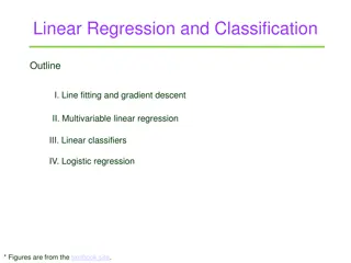
2. Regression Analysis Recall our early discussion Given a set of predictors/features, x, and an outcome of interest, y Main goal is to identify a function f(x) that predicts y well Linear regression assumes a structural relationship between x and y ( ) ( where y = XX X f X = = + + + + y ... X X X 0 1 1 2 2 p p ) 1 ' ' ols Used so often because models are simple and interpretable

3. Problems with Linear Regression OLS models fit to all predictors may inhibit interpretability Consider model selection approaches OLS model fit to all predictors may over-fit the data Results in poor generalizability Not able to predict new data well In data with many predictors, there may also be issues of collinearity That is, one or more predictors in X may be described by a linear combination of other predictors in X Certainly happens if p > n (then X is not full column rank).

4. Collinearity If the feature matric X is not full rank, a linear combination aX of columns in X =0 In such a case the columns are co-linear in which case the inverse of X X doesn t exist It is rare that aX == 0, but if a combination exists that is nearly zero, (X X)-1is numerically unstable Results in very large estimated variance of the model parameters making it difficult to identify significant regression coefficients

5. Penalized Regression Penalized regression model take the general form ( 1 i = ) 2 ( ) q n p p = + 0 M y x q q i ij j j = = 1 1 j j Some of these approaches designed to handle collinear predictors Ridge: ( ) 1 i i j M y = = ( ) 1 i i j M y = = ( ) 2 2 n p p = + 2 j x 2 ij j = 1 1 j ( ) n p p p Elastic Net: = + + 2 j x 1 2 ij j j = = 1 1 1 j j However, there are other alternatives (that require less tuning ) available

6. Derive Input Approaches for Collinearity Principal Components Regression (PCR) Define a set of p principal components Linear combinations of the original predictors in X Fit a linear regression model to these derived components Partial Least Squares Regression (PLSR) Define a set of derived inputs (latent variables) Also a linear combination of X but also accounts for y The latent variables are estimated iteratively Note, these methods are also helpful if p is large as they typically use a subset of size m < p of components

7. Defining Genetic Race by PCA Zakharia F, et al. (2009). Characterizing the admixed African Ancestry of African Americans. Genome Biology, 10(12): R141

8. Principal Component Regression (PCR) Use of PCR can serve two objectives Eliminate collinearity by developing p orthogonal derived components, z1, z2, , zp, as alternative for the original correlated pfeatures, x1, x2, , xp, in X Reduce number of features need to fit the regression model for yby including only m < p(# of original predictors) Choose the m components that capture a majority of the variability in X So how do we come up with these derived orthogonal components?

9. Exact Principal Components Our components, Z, are represented for data Xnxp as linear combinations of p random measurements on j = 1,2, ,nsubjects

10. Exact Principal Components We can also find the moments for these p linear combinations of our data X

11. Exact Principal Components We can also find the moments for these p linear combinations of our data X

12. Exact Principal Components Principal components are those combinations that are: (1) Uncorrelated (linear combinations Z1, Z2, , Zp) (2) Variance as large as possible (3) Subject to: = ' st a X 1 linearcombomaximizes PC 1 1 ( ) = ' ' a X 1 1 a a subjectto Var 1 = ' 2 1 and nd a X 2 linearcombomaximizes PC ( ) ( ) = = ' 2 ' 2 ' ' 2 a X a a a X a X subjectto , 0 Var Cov 2 1 = ' th a X linearcombomaximizes p PC p ( ) ( ) = = ' ' ' i ' a X a a a X a X subjectto 1 and , 0 f or i Var Cov p p p p p

13. Finding PCs Under Constraints So how do we find PC s that meet the constraints we just discussed? We want to maximize subject to the constraint that This constrained maximization problem can be done using the method of Lagrange multipliers Thus, for the first PC we want to maximize ( ) ( ) = = ' ' a X a a Var Z 1 Var 1 1 1 1 = ' 1 1 a a ( ) ( ) = ' ' ' ' a Ma 1 1 a a a a 1 1 a a 1 1 1 1 1 1 1

14. Finding 1st PC Under Constraints Differentiate w.r.t a1and set equal to 0 :

15. Recall Eigenvalues and Eigenvectors The eigenvalues of an Anxn matrix ... 0 1 2 p are scalar values that are the solutions to = = A I A 0 or e i i e i for a set of eigenvectors, . Typically normalized so that 1 2 , ,..., e e e p = = ' 1 ee i i ' 0 for all ee i j i j

16. Finding 2nd PC Under Constraints We can think about this in the same way, but we now have an additional constraint We want to maximize but subject to ( ) 2 Var Z = ( ) = ' 2 ' 2 a X a a Var 2 = = ' 2 ' 2 1 a a a a 1 & 0 2 So now we need to maximize ( ) ' 2 ' 2 ' 2 1 a a a a a a 1 2 2

17. Finding 2nd PC Under Constraints Differentiate w.r.t a2and set equal to 0:

18. Finding 2nd PC Under Constraints Differentiate w.r.t a2and set equal to 0:

19. Finding PCs Under Constraints But how do we choose our eigenvector (i.e. which eigenvector corresponds to which PC?) We can see that what we want to maximize is = = = ' i ' i ' i a a a a a a i i i i i i So we choose i to be as large as possible If 1 is our largest eigenvalue with corresponding eigenvector ei then the solution for our max is = a 1 1 e 1

20. Exact Principal Components So we can compute the PCs from the variance matrix of X, : ( ) X = 1. eigenvalues of Var 1 2 p e e e 2. , , , correspondingeigenvectorsof suchthat 1 2 p = = = e e e e e i i e i ' i i 1 ' i 0 i j j th This yields our principalcomponent i = = + + + ' i e X e X e X e X ... Z 1 1 2 2 i i i pi p

21. Properties We can update our moments using the proposed solution

22. Properties We can update our moments using the proposed solution

23. Properties We can update our moments using the proposed solution

24. Properties Normality assumption not required to find PC s If X ~ Np( ) then: 1 ' e Z 1 1 2 = = ' ' X ~ , N X ' e Z p p p and ,Z ,...,Z are independent Z 1 2 p Total Variance: ( ) ( ) ( ) ( ) = = + + + ... trace Var X Var X Var X 1 + 2 p + + ... 1 2 p ( ) ( ) ( ) = + + + ... Var Z Var Z Var Z 1 2 p th and proportion total variance accounted for Var Z = component k ( ) k k ( ) p p Var Z i i = = 1 1 j j

25. Principal Components Consider data with p random measures on i = 1,2, ,nsubjects For the ith subject we then have the random vector X X X 1 i 2 i = = X 1,2,..., i n i X ip ( ) = Suppose ~ , ...if we set 2 weknowwhat lookslike N p X i i X2 2 X1 1

26. Graphic Representation Now suppose X1, X2 ~ N2( , ) X2 Z1 Z2 X1 ( ) 2 n Z1axis selected to maximize variation in the scores Z2axis must be orthogonal to Z1 and maximize variation in the scores 2 2 1 i i Z Z = Z Z 1 1 i = 1 i ( ) 2 n

27. How Much Variance is Captured Proportion of total variance accounted for by the first k components is k i = 1 i p i = 1 i If the proportion of variance accounted for by the first k principal components is large, we might want to restrict our attention to only these first k components Keep in mind, components are simply linear combinations of the original p measurements

28. PCs from Standardized Variables As was the case with penalized regression, PC s are not scale invariant. Thus we want to standardize our variables before finding PCs ( ) X 1 1 11 ( ) X 2 2 ( ) ( ) 1 2 1 2 = = ' i th V X PC becomes: i Z e V X 22 i ( ) X p p pp e butnow and are the eigenvalues/vectors for andbecause they are standardized: i i ( ) ( ) p = = 1 and Var Z Var Z p i i = 1 i

29. Compare Standardized/Non-standardized PCs Non standardized ? =1 4 ?1= 100.16 ?2= 0.84 Standardized 1 0.4 ?1= 1.4 ?2= 0.6 4 0.4 1 100 ? = = 0.04 = 0.999 = 0.707 = 0.707 ?1 ?2 0.999 0.04 ?1 ?2 0.707 0.707

30. Estimation In general we do not know what is- we must estimate if from the sample So what are our estimated principal components? X Assumewehavearandomsample: We can use: S ( )( ) ' n = S X X X X 1 i i 1 n = 1 i Eigenvaluesfor : .... S (consistentestimators , ,..., ) 1 2 1 2 p p Eigenvectorsfor e : e e e e e .... (consistentestimators , ,..., ) 1 2 1 2 p p thi principa l component: z =e x ' i i

31. Back to PCR Once we have our estimated PCs, z1,z2, , zp, we want to fit a regression model for our response y using our PC as the features We can calculate the values for our new derived components for each of our n observations Based on the linear combination of our original x s described by z1, z2, , zp Note this still doesn t reduce the number of features used in our regression model If we let m = p, our estimate will be the same as OLS However, if we want to reduce the number of features in our model, we can again use a cross-validation approach

32. Software The pls package in R can fit both PCR and PLSR models The pls package has reasonable functionality for fitting models Has built in cross-validation Also has many available plotting features Loading on each xj for the derived features (a) fraction of L1-norm (b) maximum number of steps There is also a nice tutorial for the package available in the Journal of Statistical Soft

33. Body Fat Example library(pls) ### Fitting a Principal Component Model ### bf.pcr <- pcr(PBF ~ ., data=bodyfat2, validation = "CV") summary(bf.pcr) Data: X dimension: 252 13 Y dimension: 252 1 Fit method: svdpc Number of components considered: 13 VALIDATION: RMSEP Cross-validated using 10 random segments. (Intercept) 1 comps 2 comps 3 comps 4 comps 5 comps 6 comps 7 comps 8 comps 9 comps 10 comps 11 comps 12 comps 13 comps CV 1.002 0.7897 0.6888 0.6402 0.6401 0.6693 0.6410 0.6201 0.6045 0.6069 0.6080 0.6133 0.5328 0.5314 adjCV 1.002 0.7893 0.6902 0.6375 0.6392 0.6684 0.6401 0.6126 0.6023 0.6046 0.6056 0.6103 0.5309 0.5296 TRAINING: % variance explained 1 comps 2 comps 3 comps 4 comps 5 comps 6 comps 7 comps 8 comps 9 comps 10 comps 11 comps 12 comps 13 comps X 61.85 72.27 79.98 85.12 89.72 92.14 94.34 96.34 97.75 98.78 99.38 99.82 100.0 PBF 38.55 54.12 58.36 58.66 60.64 62.83 67.36 67.41 67.58 67.99 68.30 74.78 74.9

34. Examining the Model Graphically plot(bf.pcr, plottype="validation , legendpos= topright )

35. Body Fat Example names(bf.pcr) [1] "coefficients" "scores" "loadings" "Yloadings" "projection" "Xmeans" [7] "Ymeans" "fitted.values" "residuals" "Xvar" "Xtotvar" "fit.time" [13] "ncomp" "method" "validation" "call" "terms" "model round(bf.pcr$coefficients[,,1:3], 4) ### OR use coef(bf.pcr, 1:3) (Note, this returns these coefficients as an array) 1 comps 2 comps 3 comps Age 0.0022 0.2566 0.1702 Wt 0.0754 0.0693 0.0774 Ht 0.0221 -0.1367 -0.2761 Neck 0.0669 0.0973 0.0274 Chest 0.0692 0.1401 0.1527 Abd 0.0683 0.1580 0.1831 Hip 0.0714 0.0724 0.1178 Thigh 0.0679 0.0261 0.0923 Knee 0.0675 0.0507 0.0505 Ankle 0.0505 -0.0255 -0.0518 Bicep 0.0655 0.0489 0.0644 Arm 0.0547 0.0092 -0.0053 Wrist 0.0611 0.0885 0.0087

36. Body Fat Example round(bf.pcr$scores, 3) ### OR use scores(bf.pcr) Comp1 Comp2 Comp3 Comp4 Comp5 Comp6 Comp7 Comp8 Comp9 Comp10 Comp11 Comp12 Comp13 1 -2.220 1.237 -1.496 -0.285 0.163 -0.236 -0.226 0.263 -0.076 -0.292 0.153 -0.364 -0.037 2 -0.886 2.010 -0.038 -0.228 -0.168 -0.745 -0.050 -0.609 -0.192 0.165 -0.220 0.030 0.039 3 -2.361 1.220 -2.194 1.914 -0.181 0.264 0.166 -0.129 0.073 -0.438 0.114 -0.153 -0.291 249 2.640 -2.313 1.304 0.073 -0.045 -0.379 -0.787 0.211 0.244 -0.211 -0.203 -0.148 -0.046 250 0.451 -3.206 -0.472 0.288 1.008 -0.179 0.713 -0.061 0.086 0.345 0.334 -0.263 0.046 251 1.235 -2.183 1.811 0.154 -0.122 0.557 -0.447 -0.989 0.263 -0.735 0.204 -0.188 0.166 252 3.693 -2.370 1.799 0.406 -0.773 -0.025 -0.604 -0.633 0.584 -0.310 -0.234 -0.127 -0.186

37. Body Fat Example bf.pcr$loadings ### OR use loadings(bf.pcr) Loadings: Comp1 Comp2 Comp3 Comp4 Comp5 Comp6 Comp7 Comp8 Comp9 Comp10 Comp11 Comp12 Comp13 Age -0.751 0.420 0.294 0.207 -0.152 0.262 0.166 Wt 0.345 0.142 -0.206 0.190 0.872 Ht 0.101 0.469 0.678 0.485 0.115 0.134 0.102 0.124 Neck 0.306 0.121 -0.206 -0.561 -0.115 -0.703 Chest 0.316 -0.209 0.152 0.450 0.248 -0.431 0.398 0.409 -0.214 Abd 0.312 -0.265 -0.122 0.120 0.229 0.295 0.140 -0.791 Hip 0.326 -0.221 0.178 0.163 -0.101 0.134 0.323 -0.609 0.343 -0.403 Thigh 0.310 0.123 -0.322 -0.273 -0.115 0.522 0.631 Knee 0.308 0.247 0.497 -0.443 -0.137 -0.272 -0.540 Ankle 0.231 0.224 0.128 0.500 -0.679 0.347 0.167 -0.106 Bicep 0.299 -0.322 -0.150 0.845 0.129 -0.147 -0.110 Arm 0.250 0.134 -0.683 -0.310 0.446 0.228 -0.273 0.153 Wrist 0.279 0.388 -0.265 -0.352 -0.467 -0.272 0.513

38. Body Fat Example round(bf.pcr$loadings[,1:13], 3) Loadings: Comp1 Comp2 Comp3 Comp4 Comp5 Comp6 Comp7 Comp8 Comp9 Comp10 Comp11 Comp12 Comp13 Age 0.010 -0.751 0.420 0.079 -0.040 0.294 -0.034 0.207 -0.152 0.262 0.031 0.166 0.041 Wt 0.345 0.018 -0.039 0.087 0.142 -0.031 0.076 -0.047 0.061 -0.019 -0.206 0.190 0.872 Ht 0.101 0.469 0.678 0.082 0.485 0.115 0.134 0.102 0.005 0.124 0.062 -0.008 -0.090 Neck 0.306 -0.090 0.121 -0.206 0.055 -0.561 0.007 -0.115 -0.703 -0.048 -0.073 -0.013 -0.095 Chest 0.316 -0.209 -0.061 -0.009 0.152 -0.070 0.450 -0.061 0.248 -0.431 0.398 0.409 -0.214 Abd 0.312 -0.265 -0.122 0.120 0.229 0.033 0.295 -0.086 0.140 0.086 -0.037 -0.791 -0.046 Hip 0.326 -0.003 -0.221 0.178 0.163 0.045 -0.049 -0.101 0.134 0.323 -0.609 0.343 -0.403 Thigh 0.310 0.123 -0.322 0.077 0.096 0.062 -0.273 0.041 -0.115 0.522 0.631 0.073 0.018 Knee 0.308 0.050 0.001 0.247 0.005 0.497 -0.443 -0.137 -0.272 -0.540 -0.013 -0.088 -0.076 Ankle 0.231 0.224 0.128 0.500 -0.679 -0.032 0.347 0.167 -0.106 0.080 0.011 -0.024 -0.035 Bicep 0.299 0.049 -0.076 -0.322 -0.035 -0.045 -0.150 0.845 0.129 -0.147 -0.110 -0.081 -0.049 Arm 0.250 0.134 0.071 -0.683 -0.310 0.446 0.228 -0.273 -0.035 0.153 -0.043 -0.005 -0.002 Wrist 0.279 -0.081 0.388 -0.059 -0.265 -0.352 -0.467 -0.272 0.513 0.007 0.071 -0.077 -0.030

39. Body Fat Example bf.pcr$Yloadings Loadings: Comp1 Comp2 Comp3 Comp4 Comp5 Comp6 Comp7 Comp8 Comp9 Comp10 Comp11 Comp12 Comp13 PBF 0.219 -0.339 -0.206 0.181 0.264 0.398 0.176 0.197 -1.067 -0.227 Comp1 Comp2 Comp3 Comp4 Comp5 Comp6 Comp7 Comp8 Comp9 Comp10 Comp11 SS loadings 0.048 0.115 0.042 0.005 0.033 0.070 0.158 0.002 0.009 0.031 0.039 Proportion Var 0.048 0.115 0.042 0.005 0.033 0.070 0.158 0.002 0.009 0.031 0.039 Cumulative Var 0.048 0.163 0.205 0.210 0.243 0.313 0.471 0.473 0.482 0.513 0.552 Comp12 Comp13 SS loadings 1.139 0.052 Proportion Var 1.139 0.052 Cumulative Var 1.691 1.743 round(as.vector(bf.pcr$Yloadings), 4) [1] 0.2190 -0.3389 -0.2057 0.0675 0.1815 0.2643 0.3978 0.0458 0.0954 0.1758 0.1973 -1.0672 -0.2275

40. Body Fat Example So what exactly are the coefficients in a pcr R object?

41. Body Fat Example So what exactly are the coefficients in a pcr R object?

42. Body Fat Example So what exactly are the coefficients in a pcr R object?

43. Examining the Model Graphically plot(bf.pcr, plottype= coef , 1:3, legendpos= bottomright )

44. Examining the Model Graphically plot(bf.pcr, plottype= loadings , 1:3, legendpos= bottomright ) loadingplot(bf.pcr, 1:3)

45. Examining the Model Graphically par(mfrow=c(2,2)) plot(bf.pcr, "prediction", ncomp=1); plot(bf.pcr, "prediction", ncomp=4) plot(bf.pcr, "prediction", ncomp=8); plot(bf.pcr, "prediction", ncomp=13)

46. Examining the Model Graphically plot(bf.pcr, score , 1:3)

47. Examining the Model Graphically plot(bf.pcr, plottype="correlation", pch=16, col=c(1:8,"yellow","wheat","purple","goldenrod","skyblue"), cex=2) legend(x=0.95, y=1.10, legend=colnames(bodyfat[,2:14]), col=c(1:8,"yellow","wheat","purple","goldenrod","skyblue"), cex=0.8, pch=16, bty="n")

48. Examining the Model Graphically plot(bf.pcr, plottype="correlation", 1:4, pch=16, col=2)

49. Comparison to OLS? ### Comparison to OLS fit bf.ols<-lm(PBF ~ ., data=bodyfat2) pbf.ols<-predict(bf.ols) bf.pcr <- pcr(PBF ~ ., data=bodyfat2, validation = "CV") pbf3<-fitted(bf.pcr, ncomp=3)[,,3] pbf.fullpcr<-fitted(bf.pcr, ncomp=13)[,,13] plot(pbf.ols, pbf.fullpcr, xlab="predictions from OLS", ylab="predictions from full PCR", pch=16, col=3) points(pbf.ols, pbf3, pch=1, col=2)

50. Partial Least Square Regression (PLSR) Similar to PCR with some important differences Also eliminates collinearity using a derived set of orthoganol components, z1, z2, , zm, BUT, PLSR used both the original correlated pfeatures, x1, x2, , xp, in X and response vectory Thus components include information on the variability in X But also include information on the correlation between X andy As in PCR, reduce the number of features need to fit the regression model for yby including only m< pof the original predictors These components that depend on both Xand y are estimated iteratively

Load More ...