Arctic Sea Ice Regression Modeling & Rate of Decline
 undefined


Rate of Decline of the
Arctic Sea Ice and
Regression Modeling
PRESENTER: AMANDA WALKER
TEXAS STATE UNIVERSITY


Melting Sea Ice
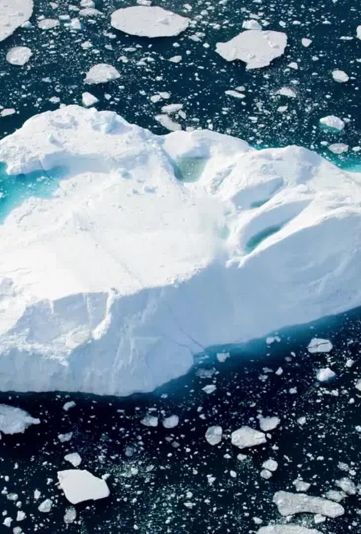

Variables:
Explanatory: Year (measurements begin in 1979)
Response: Arctic Sea Ice Extent (surface area in million
square km)
https://climate.nasa.gov/vital-signs/arctic-sea-ice/
Modeling Linear Regression
Scatterplot,
LSRL, interpret
slope
Interpret Scatterplot
Write the LSRL: y = 167.01 – 0.080601x
Correlation coefficient r = -0.89225
Interpret Slope as a rate of change*
- Each year since 1979 the extent of artic sea ice decreases
by 80,601 km squared, on average!
Interpret Residual Plot
Interpreting residual plot can be a bit tricky for students at first, especially since
R includes the polynomial fit.
There is potential curvature of the residuals around the line y=0, which might
indicate a quadratic model is more appropriate.
Transform Data for
Quadratic Regression
Right click on the data set, select Function,
Select Transform
Create Variable: Quad
Returned Variable: Year^2
Save this new Data Set: New Arctic
Multiple
Linear
Regression
Using this
new Data Set
Compare
Residual Plots &
Coefficient of
Determination
for each model
Quadratic: R-squared 0.805671
Linear: R-squared: 0.79611
While these are close, the quadratic model has less
curvature around the line y=0 and higher R-squared value.
*Note: I recently updated this data set using new
measurements from NASA and the R-squared values have
gotten closer over the last two years.
Resources:
This lesson was adapted from the article published in JSE (Witt
2013)
Witt, G. (2013). Using Data from Climate Science to Teach
Introductory Statistics.
Journal of Statistics Education, 21
(1),
http://jse.amstat.org/v21n1/witt.pdf
https://climate.nasa.gov/vital-signs/arctic-sea-ice/
Explore the rate of decline of Arctic sea ice through regression modeling techniques. The presentation covers variables, linear regression, interpretation of scatterplots and residual plots, quadratic regression, and the comparison of models. Discover the decreasing trend in Arctic sea ice extent since 1979 and the implications of the findings.

Uploaded on Sep 07, 2024 | 1 Views
Download Presentation

Please find below an Image/Link to download the presentation.
The content on the website is provided AS IS for your information and personal use only. It may not be sold, licensed, or shared on other websites without obtaining consent from the author.If you encounter any issues during the download, it is possible that the publisher has removed the file from their server.
You are allowed to download the files provided on this website for personal or commercial use, subject to the condition that they are used lawfully. All files are the property of their respective owners.
The content on the website is provided AS IS for your information and personal use only. It may not be sold, licensed, or shared on other websites without obtaining consent from the author.
E N D
Presentation Transcript
Rate of Decline of the Arctic Sea Ice and Regression Modeling PRESENTER: AMANDA WALKER TEXAS STATE UNIVERSITY
Melting Sea Ice Variables: Explanatory: Year (measurements begin in 1979) Response: Arctic Sea Ice Extent (surface area in million square km) https://climate.nasa.gov/vital-signs/arctic-sea-ice/
Modeling Linear Regression I have taught this lesson using fathom, JMP, and once with the TI calculator where I asked students to enter data into calculator before coming to class. This presentation uses Rguroo, and internet based statistical software.
Interpret Scatterplot Write the LSRL: y = 167.01 0.080601x Scatterplot, LSRL, interpret slope Correlation coefficient r = -0.89225 Interpret Slope as a rate of change* - Each year since 1979 the extent of artic sea ice decreases by 80,601 km squared, on average!
Interpret Residual Plot Interpreting residual plot can be a bit tricky for students at first, especially since R includes the polynomial fit. There is potential curvature of the residuals around the line y=0, which might indicate a quadratic model is more appropriate.
Transform Data for Quadratic Regression Right click on the data set, select Function, Select Transform Create Variable: Quad Returned Variable: Year^2 Save this new Data Set: New Arctic
Multiple Linear Regression Using this new Data Set
Quadratic: R-squared 0.805671 Compare Residual Plots & Coefficient of Determination for each model Linear: R-squared: 0.79611 While these are close, the quadratic model has less curvature around the line y=0 and higher R-squared value. *Note: I recently updated this data set using new measurements from NASA and the R-squared values have gotten closer over the last two years.
Resources: This lesson was adapted from the article published in JSE (Witt 2013) Witt, G. (2013). Using Data from Climate Science to Teach Introductory Statistics. Journal of Statistics Education, 21(1), http://jse.amstat.org/v21n1/witt.pdf https://climate.nasa.gov/vital-signs/arctic-sea-ice/