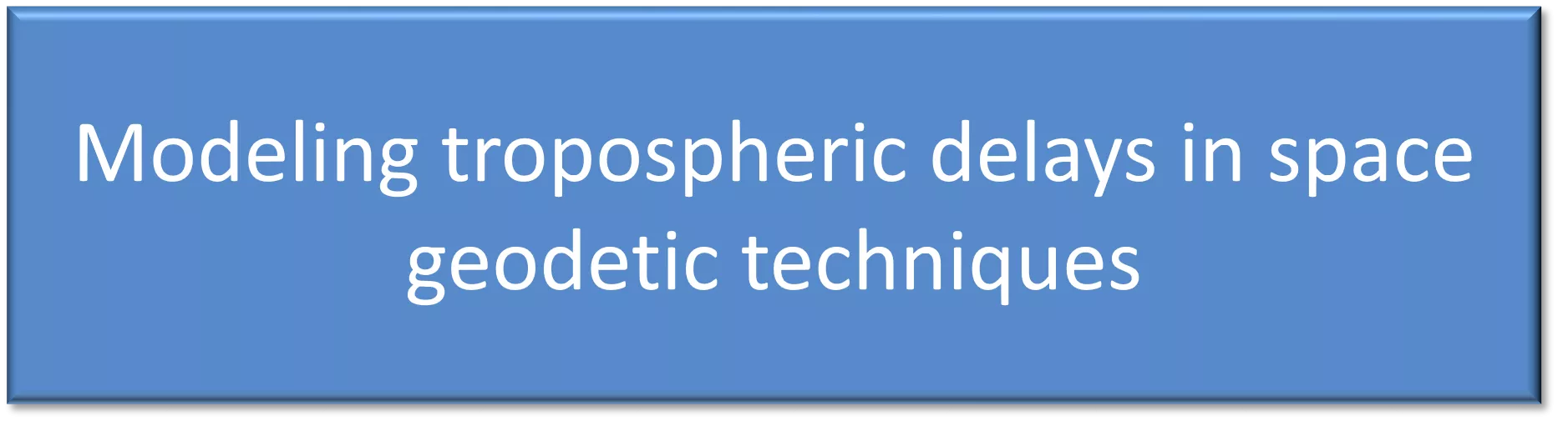
Tropospheric Delays in Geodetic Techniques


Daniel Landskron


GEOWEB Training course on modern geodetic topics
Mostar, Bosnia and Herzegovina
October 16, 2017


1.
Fundamentals
2.
Modeling delays in the troposphere
3.
Vienna troposphere models
4.
Conclusion
5.
Outlook
2
3
•
Troposphere delays: strictly speaking delays in the
neutral atmosphere (up to 100 km)
•
Radio signals are delayed and bent due to interaction
with gases and water particles => refractivity
•
Essentially no frequency dependence across
microwave regime
•
Small frequency dependence for optical techniques
(Satellite Laser Ranging)
4
•
Strictly speaking, refractivity is a complex number
•
Real part: causes refraction and propagation delays
•
Imaginary part: causes absorption; important for
water vapour radiometers
5
6
Distinguished between a hydrostatic part and a wet part
7
hydrostatic
wet
Wet part: surface values not representative for the
upper air conditions
8
•
k
3
can be ignored; Wet part smaller
•
Small frequency-dependency
9
10
11
Bending effect [S - G] about 0.2 m at 5°
elevation (added to the hydrostatic mapping
function)
•
Zenith hydrostatic delay
–
Ca. 2.3 m at sea level
–
Can be determined very accurately from
p
(mm-accuracy)
+ Saastamoinen (1972)
•
Zenith wet delay
–
Ca. 0.05 - 0.4 m at sea level
–
Rule of thumb:
–
Can only be approximated from surface data
GPT2/GPT3 + Askne & Nordius (1987)
12
•
Simple empirical models like Berg (1948) and Hopfield
(1969)
•
More sophisticated models like
–
UNB3m (5 latitude bands, annual with fixed phase)
–
GPT (9x9 spherical harmonics, annual with fixed phase)
–
GPT2/GPT3 (5°x5° or 1°x1° grid, annual + semi-annual
terms)
13
14
•
Integrated water vapour IWV in kg/m
2
•
Precipitable water PW in m
•
PW is approximately 1/6 of the zenith wet delay
15
16
Comparison of IWV for station
MATERA
17
ΔL(e)
: total delay dependent on elevation
ΔL
z
h
: hydrostatic delay in zenith direction; can be modeled a priori
ΔL
z
w
: wet delay in zenith direction; approximated or estimated in
data analysis
mf(e)
: mapping function (
mf
h
>
mf
w
)
Assuming Azimuthal Symmetry:
•
Mapping function not perfectly known
•
Errors via correlations also in station heights (and
clocks)
•
Low elevations necessary to de-correlate heights,
clocks, and zenith delays
•
Rule of thumb: the station height error is about 1/5
of the delay error at 5°elevation (if cutoff angle is 5°)
18
•
Continued fraction form (Herring, 1992)
19
•
Saastamoinen (1972), Chao (1974), CfA2.2 (Davis et
al., 1985), ...
•
MTT
: MIT Temperature mapping functions (Herring,
1992)
•
NWF
: New Mapping Functions (Niell, 1996)
•
IMF
: Isobaric Mapping Functions (Niell, 2000)
•
VMF
: Vienna Mapping Functions (Böhm et al., 2006)
•
GMF
: Global Mapping Functions (Böhm et al., 2006)
•
GPT2/GPT2w
(Lagler et al., 2013, Böhm et al., 2015)
•
VMF3/GPT3
(Landskron and Böhm, 2017)
20
21
ΔL(a,e)
: total delay dependent on azimuth and elevation (m)
ΔL
z
: delay in zenith direction (m)
mf(e)
: mapping function
G
n
: north gradient (m)
G
e
: east gradient (m)
Assuming Azimuthal Asymmetry:
•
Horizontal gradients due to:
–
Atmospheric bulge
–
Weather fronts
–
Coastal conditions
•
Chen and Herring (1997)
C
h
= 0.0031,
C
w
= 0.0007
•
Typical gradient: 1 mm (corresponds to 0.1 m delay at 5°
elevation)
22
•
Correspond to tilting of the mapping function
23
Gradients are either estimated in the analysis or they are
determined from external data (e.g. NWM)
A priori models:
•
DAO
(MacMillan and Ma, 1997)
•
LHG
(Böhm and Schuh, 2007)
•
APG
(Böhm et al., 2013)
•
GRAD
(Landskron et al., 2016)
•
GPT3
(Landskron et al., 2017)
24
•
To find the ray-path from the source to the telescope
(iterative calculation)
•
Coupled differential equations need to be solved
•
1D, 2D or 3D ray-tracing
•
Feasible for VLBI but probably not for GNSS
•
Basis for most accurate mapping functions and
gradient models (VMF series)
25
26
n=1
•
WVR estimate the wet delay by measuring the
thermal radiation from the sky
•
At microwave frequencies where the atmospheric
attenuation due to water vapour is rather high
•
WVR do not work during rain or below 15° elevation
27
Konrad (Elgered
et al., 2012)
•
Wet part much smaller than for microwaves
•
Only modeled, not estimated
•
Thus, better estimation of height compared to
horizontal components
•
Theoretical possibility to estimate troposphere delay
with two frequencies, but accuracy of delays not yet
sufficient for that
28
•
Atmospheric Effects in Space
Geodesy, Böhm and Schuh (2013)
•
Very detailed description of
tropospheric delays
29
30
•
TU Wien has become main provider of troposphere
models
•
Applicable for GNSS and VLBI analysis
•
Included in important software as well as realizations
(Bernese, ITRF,..)
31
32
•
Plane wavefronts because of
huge distance (~10 billion ly)
•
Determine phase difference
τ
between 2 sites
•
Correct for errors (ionosphere,
troposphere,..)
Station positions and
velocities, source positions,
zenith wet delay
•
Discrete mapping functions
VMF
: Vienna Mapping Functions (Böhm and Schuh, 2004)
VMF1
: Vienna Mapping Functions 1 (Böhm et al., 2006)
VMF3
: Vienna Mapping Functions 3 (Landskron and Böhm, 2017)
•
Empirical mapping functions
GMF
: Global Mapping Functions (Böhm et al., 2006)
GPT
: Global Pressure and Temperature (Böhm et al., 2007)
GPT2w
: Global Pressure and Temperature 2 (Lagler et al., 2013)
GPT2w
: Global Pressure and Temperature 2 wet (Böhm et al., 2015)
GPT3
: Global Pressure and Temperature 3 (Landskron and Böhm, 2017)
•
Hybrid Model
SA-GPT2w
: Site-Augmented GPT2w (Landskron et al., 2015)
33
http://ggosatm.hg.tuwien.ac.at
34
•
Determined from ray-traced delays through NWM
from ECMWF
•
Empirical functions for
b
and
c
coefficients
•
All information from ray-tracing is condensed into
the
a
coefficients
•
Available 6-hourly, either at VLBI/GNSS stations or on
a global grid
35
36
37
38
Spherical harmonics expansion for coefficients
b
and
c
up to degree and order 12
•
GMF: “Averaged” VMF
•
Spherical Harmonics up to degree and order 9 for
a
,
b
and
c
from VMF1
•
Annual variation with fixed phase (January 28)
39
•
Refined combination of GMF and GPT + additional
parameters
•
Not based on spherical harmonics, but on a grid-wise
representation
•
Bilinear interpolation from grid to desired location
40
41
42
Data fitting in order to derive
empirical information
a
h
: mean value and annual variation
43
44
mjd
lat
lon
h
ell
a
h
a
w
mjd
lat
lon
zd
VMF3
mf
h
mf
w
GPT3
a
h
a
w
p T dT Tm e
λ
N G
n
h
G
e
h
G
n
w
G
e
w
45
46
47
VMF1
VMF3
Differences in slant total delay to ray-tracing (mm)
2592 grid points
120 epochs (2001-2010)
el
= 5°
Differences in slant total delay to ray-tracing (mm)
2592 grid points
120 epochs (2001-2010)
el
= 5°
48
GPT2w
GPT3
49
Mean absolute error (MAE) in slant delay w.r.t. ray-tracing (mm)
2592 grid points
120 epochs (2001-2010)
el
= 5°
50
Mean absolute diff in slant total delay
w.r.t. ray-tracing (mm)
33 sites around the world
1999-2014
51
Mean difference w.r.t. ray-tracing (mm)
33 sites around the world, 1999-2014, el =5°
shd
swd
VMF1
VMF3
52
•
Baseline Length Repeatability (BLR) from VLBI analysis
good tool for assessing accuracy of geodetic products
•
Analysis with Vienna VLBI and Satellite Software
(VieVS)
•
Hardly any difference between the mapping function
models
•
Main influence from zenith delays, mapping functions
not that effective
•
Estimation of zenith wet delays very accurate
53
1.
Empirical from GPT2w
2.
Measure
T
and
e
in situ
3.
Augment the empirical
54
1. VMF3
2. GPT3
3. SA-GPT2w
T
with
Δ
L
w
z
: 0.65
e
with
Δ
L
w
z
: 0.85
Universal, global coefficients
M
1
,
M
2
:
M
1
=
4.9 * 10
-4
[m/°C
-1
]
M
2
=
0.00915
[m/hPa
-1
]
Refined and site-augmented tropospheric delay models for GNSS applications (Landskron et al., 2016)
55
2016/02/10
Comparison of
Δ
L
w
z
for
BZRG
IGS
GPT2w
GPT2w + T
GPT2w + T, e
Refined and site-augmented tropospheric delay models for GNSS applications (Landskron et al., 2016)
56
2016/02/10
Comparison of
Δ
L
w
z
for
BZRG
IGS
GPT2w
GPT2w + T
GPT2w + T, e
Refined and site-augmented tropospheric delay models for GNSS applications (Landskron et al., 2016)
57
2016/02/10
Comparison of
Δ
L
w
z
for
BZRG
IGS
GPT2w
GPT2w + T
GPT2w + T, e
Refined and site-augmented tropospheric delay models for GNSS applications (Landskron et al., 2016)
58
2016/02/10
Comparison of
Δ
L
w
z
for
ALIC
IGS
GPT2w
GPT2w + T
GPT2w + T, e
Refined and site-augmented tropospheric delay models for GNSS applications (Landskron et al., 2016)
59
2016/02/10
Comparison of
Δ
L
w
z
for
ALIC
IGS
GPT2w
GPT2w + T
GPT2w + T, e
Refined and site-augmented tropospheric delay models for GNSS applications (Landskron et al., 2016)
60
2016/02/10
Comparison of
Δ
L
w
z
for
ALIC
IGS
GPT2w
GPT2w + T
GPT2w + T, e
Refined and site-augmented tropospheric delay models for GNSS applications (Landskron et al., 2016)
61
2016/02/10
Comparison of
Δ
L
w
z
for
NYA1
IGS
GPT2w
GPT2w + T
GPT2w + T, e
Refined and site-augmented tropospheric delay models for GNSS applications (Landskron et al., 2016)
62
2016/02/10
Comparison of
Δ
L
w
z
for
NYA1
IGS
GPT2w
GPT2w + T
GPT2w + T, e
Refined and site-augmented tropospheric delay models for GNSS applications (Landskron et al., 2016)
63
2016/02/10
Comparison of
Δ
L
w
z
for
NYA1
IGS
GPT2w
GPT2w + T
GPT2w + T, e
64
Mean absolute error (MAE) in zenith wet delay to ray-
tracing (cm)
33 sites around the world
1999-2014
65
•
GPT2w well suited for site-augmented approach using in
situ measurements of
T
and
e
•
in situ measurement of
T
yields small improvement in
zenith wet delay
Δ
L
w
z
(~5%)
•
additional in situ measurement of
e
yields significant
improvement in zenith wet delay
Δ
L
w
z
(~30%)
•
In general, best performance of site-augmented GPT2w
is
achieved in dry regions
•
Discrete a priori gradient models
LHG
: Linear Horizontal Gradients (Böhm and Schuh, 2007)
GRAD
(Landskron et al., 2016)
•
Empirical a priori gradient models
APG
: A priori gradients (Böhm et al., 2013)
GPT3
: Global Pressure and Temperature 3 (Landskron and Böhm, 2017)
66
http://ggosatm.hg.tuwien.ac.at
67
= GRAD-1
= GRAD-2
•
Determined from 2D-raytracing at 7 elevations and 16 azimuths
through LSM
•
For all VLBI measurements
•
6-hourly (at each NWM epoch)
68
No gradients
GRAD-1
GRAD-2
GRAD-3
Residuals between ray-traced delays and modeled delays
69
Higher-order gradients smaller in size
WETTZELL, September 2011
Higher-order gradients improve delays
WETTZELL, September 2011
70
71
72
Empirical gradients only describe a fraction of the real gradients
WETTZELL, 06/2014–12/2014
73
Mean absolute residuals (mm) between ray-tracing and
VMF3 + gradient models at el = 5°
74
Baseline length repeatability (BLR) from
1338 VLBI sessions from 2006-2014
•
GRAD yield best performance of all a priori gradients
•
Use of a priori gradients in VLBI analysis is very
important
•
Estimation only makes sense when enough
observations
•
Empirical gradients may be valuable for GNSS
75
76
•
Many troposphere models from TU Wien
•
Mapping functions + horizontal gradients
•
Applicable for GNSS and VLBI analysis
•
VMF1 and GMF most important ones
•
Ray-tracing through NWM best approach
77
78
•
Several new/refined models created
Mapping functions + horizontal gradients
All of which outperform predecessors, but only to a small
degree
•
Tropospheric modeling close to peak of technical means?
(Reference) ray-traced delays approximated very well
Denser and more accurate NWM
Improved strategies and concepts
79
•
Operationally provide VMF3/GRAD
for all IVS stations (VLBI)
for all IGS stations (GNSS)
for all IDS stations (DORIS)
on a grid
for Satellite Laser Ranging (SLR)
•
Distribute all data via:
80
http://ggosatm.hg.tuwien.ac.at
Explore the fundamentals of troposphere delays in geodetic measurements, including refractivity, modeling techniques, and impact on positioning accuracy. Discover the complexities of radio signal delays and bending effects due to atmospheric interactions. Gain insights into the Vienna troposphere models and optical refractivity variations, crucial for accurate geodetic data analysis.

Download Presentation

Please find below an Image/Link to download the presentation.
The content on the website is provided AS IS for your information and personal use only. It may not be sold, licensed, or shared on other websites without obtaining consent from the author.If you encounter any issues during the download, it is possible that the publisher has removed the file from their server.
You are allowed to download the files provided on this website for personal or commercial use, subject to the condition that they are used lawfully. All files are the property of their respective owners.
The content on the website is provided AS IS for your information and personal use only. It may not be sold, licensed, or shared on other websites without obtaining consent from the author.
E N D
Presentation Transcript
GEOWEB Training course on modern geodetic topics Mostar, Bosnia and Herzegovina October 16, 2017 Modeling tropospheric delays in space geodetic techniques Daniel Landskron
Contents 1. Fundamentals 2. Modeling delays in the troposphere 3. Vienna troposphere models 4. Conclusion 5. Outlook 2
Troposphere Troposphere delays: strictly speaking delays in the neutral atmosphere (up to 100 km) Radio signals are delayed and bent due to interaction with gases and water particles => refractivity Essentially no frequency dependence across microwave regime Small frequency dependence for optical techniques (Satellite Laser Ranging) 4
Refractivity Strictly speaking, refractivity is a complex number Real part: causes refraction and propagation delays Imaginary part: causes absorption; important for water vapour radiometers 5
Refractivity of microwaves Distinguished between a hydrostatic part and a wet part hydrostatic wet 7
Refractivity of microwaves Wet part: surface values not representative for the upper air conditions 8
Optical refractivity of moist air k3can be ignored; Wet part smaller Small frequency-dependency 9
Definition of path delay in the neutral atmosphere Bending effect [S - G] about 0.2 m at 5 elevation (added to the hydrostatic mapping function) 11
Delays in zenith direction Zenith hydrostatic delay Ca. 2.3 m at sea level Can be determined very accurately from p (mm-accuracy) + Saastamoinen (1972) Zenith wet delay Ca. 0.05 - 0.4 m at sea level Rule of thumb: Can only be approximated from surface data GPT2/GPT3 + Askne & Nordius (1987) 12
Pressure values Simple empirical models like Berg (1948) and Hopfield (1969) More sophisticated models like UNB3m (5 latitude bands, annual with fixed phase) GPT (9x9 spherical harmonics, annual with fixed phase) GPT2/GPT3 (5 x5 or 1 x1 grid, annual + semi-annual terms) 13
Precipitable water Integrated water vapour IWV in kg/m2 Precipitable water PW in m PW is approximately 1/6 of the zenith wet delay 15
Water vapor comparison Comparison of IWV for station MATERA 16
Modeling troposphere delays Assuming Azimuthal Symmetry: L(e): total delay dependent on elevation Lzh: hydrostatic delay in zenith direction; can be modeled a priori Lzw: wet delay in zenith direction; approximated or estimated in data analysis mf(e): mapping function (mfh> mfw) 17
Mapping functions Mapping function not perfectly known Errors via correlations also in station heights (and clocks) Low elevations necessary to de-correlate heights, clocks, and zenith delays Rule of thumb: the station height error is about 1/5 of the delay error at 5 elevation (if cutoff angle is 5 ) 18
Mapping functions Continued fraction form (Herring, 1992) 19
Mapping function models Saastamoinen (1972), Chao (1974), CfA2.2 (Davis et al., 1985), ... MTT: MIT Temperature mapping functions (Herring, 1992) NWF: New Mapping Functions (Niell, 1996) IMF: Isobaric Mapping Functions (Niell, 2000) VMF: Vienna Mapping Functions (B hm et al., 2006) GMF: Global Mapping Functions (B hm et al., 2006) GPT2/GPT2w (Lagler et al., 2013, B hm et al., 2015) VMF3/GPT3 (Landskron and B hm, 2017) 20
Modeling troposphere delays Assuming Azimuthal Asymmetry: L(a,e): total delay dependent on azimuth and elevation (m) Lz: delay in zenith direction (m) mf(e): mapping function Gn: north gradient (m) Ge: east gradient (m) 21
Horizontal gradients Horizontal gradients due to: Atmospheric bulge Weather fronts Coastal conditions Chen and Herring (1997) Ch= 0.0031, Cw= 0.0007 Typical gradient: 1 mm (corresponds to 0.1 m delay at 5 elevation) 22
Horizontal gradients Correspond to tilting of the mapping function 23
Horizontal gradient models Gradients are either estimated in the analysis or they are determined from external data (e.g. NWM) A priori models: DAO (MacMillan and Ma, 1997) LHG (B hm and Schuh, 2007) APG (B hm et al., 2013) GRAD (Landskron et al., 2016) GPT3 (Landskron et al., 2017) 24
Ray-tracing To find the ray-path from the source to the telescope (iterative calculation) Coupled differential equations need to be solved 1D, 2D or 3D ray-tracing Feasible for VLBI but probably not for GNSS Basis for most accurate mapping functions and gradient models (VMF series) 25
Ray-tracing n=1 26
Water vapour radiometry WVR estimate the wet delay by measuring the thermal radiation from the sky At microwave frequencies where the atmospheric attenuation due to water vapour is rather high WVR do not work during rain or below 15 elevation Konrad (Elgered et al., 2012) 27
Atmospheric delays for SLR Wet part much smaller than for microwaves Only modeled, not estimated Thus, better estimation of height compared to horizontal components Theoretical possibility to estimate troposphere delay with two frequencies, but accuracy of delays not yet sufficient for that 28
Textbook Atmospheric Effects in Space Geodesy, B hm and Schuh (2013) Very detailed description of tropospheric delays 29
Vienna models TU Wien has become main provider of troposphere models Applicable for GNSS and VLBI analysis Included in important software as well as realizations (Bernese, ITRF,..) 31
VLBI Plane wavefronts because of huge distance (~10 billion ly) Determine phase difference between 2 sites Correct for errors (ionosphere, troposphere,..) Station positions and velocities, source positions, zenith wet delay 32
Mapping functions Discrete mapping functions VMF: Vienna Mapping Functions (B hm and Schuh, 2004) VMF1: Vienna Mapping Functions 1 (B hm et al., 2006) VMF3: Vienna Mapping Functions 3 (Landskron and B hm, 2017) Empirical mapping functions GMF: Global Mapping Functions (B hm et al., 2006) GPT: Global Pressure and Temperature (B hm et al., 2007) GPT2w: Global Pressure and Temperature 2 (Lagler et al., 2013) GPT2w: Global Pressure and Temperature 2 wet (B hm et al., 2015) GPT3: Global Pressure and Temperature 3 (Landskron and B hm, 2017) Hybrid Model SA-GPT2w: Site-Augmented GPT2w (Landskron et al., 2015) http://ggosatm.hg.tuwien.ac.at 33
Vienna Mapping Functions Determined from ray-traced delays through NWM from ECMWF Empirical functions for b and c coefficients All information from ray-tracing is condensed into the a coefficients Available 6-hourly, either at VLBI/GNSS stations or on a global grid 35
Vienna Mapping Functions variable in time and space ray-tracing analytical functions 36
VMF1 vs. VMF3 VMF1 VMF3 b, c b, c from 3 years of data on a 10 x10 grid from 10 years of data on a 2.5 x2.0 grid lat. and lon. dep. for bh, bw, ch and cwthrough spherical harmonics (n=m=12) lat. dep. for ch annual and semi-annual terms for bh, bw, chand cw a annual variation for ch a LSM for el = [3 , 5 , 7 , 10 , 15 , 30 , 70 ] strictly for el = 3.3 2D ray-tracer RADIATE (Hofmeister, 2016) simple 1D ray-tracer 37
Vienna Mapping Functions 3 Spherical harmonics expansion for coefficients b and c up to degree and order 12 38
Global Mapping Functions (GMF) GMF: Averaged VMF Spherical Harmonics up to degree and order 9 for a, b and c from VMF1 Annual variation with fixed phase (January 28) 39
Global Pressure and Temperature 2 (GPT2) Refined combination of GMF and GPT + additional parameters Not based on spherical harmonics, but on a grid-wise representation Bilinear interpolation from grid to desired location 40
GPT2w vs. GPT3 GPT2w GPT3 b, c b, c from VMF1 from VMF3 a a 1 x1 or 5 x5 grid 1 x1 or 5 x5 grid annual and semi-annual terms annual and semi-annual terms mf height correction by Niell (1996) for hydr. part new mf height correction for hydr. and wet part - horizontal gradients grid 2D ray-tracer RADIATE (Hofmeister, 2016) 1D ray-tracer ECMWF monthly means 2001-2010 ECMWF monthly means 2001-2010 41
Global Pressure and Temperature 3 Data fitting in order to derive empirical information ah: mean value and annual variation 42
Handling for user GPT3 mjd lat lon hell ahawp T dT Tm e N Gnh Geh Gnw Gew VMF3 ah aw mjd lat lon zd mfh mfw 44
Delay comparison Differences in slant total delay to ray-tracing (mm) 2592 grid points 120 epochs (2001-2010) el = 5 VMF1 VMF3 47
Delay comparison Differences in slant total delay to ray-tracing (mm) 2592 grid points 120 epochs (2001-2010) el = 5 GPT2w GPT3 48
Delay comparison Mean absolute error (MAE) in slant delay w.r.t. ray-tracing (mm) 2592 grid points 120 epochs (2001-2010) el = 5 (mm) L Lh 1.67 Lw 0.30 VMF1 1.73 VMF3 0.82 0.73 0.30 GPT2w 6.85 6.10 1.63 GPT3 6.46 5.68 1.60 49
Delay comparison Mean absolute diff in slant total delay w.r.t. ray-tracing (mm) 33 sites around the world 1999-2014 [mm] 3 5 7 10 VMF1 0.52 3.98 2.54 1.47 VMF3 1.17 2.64 1.66 0.91 GPT2w (1 x1 ) 54.13 18.95 8.35 3.27 GPT3 (1 x1 ) 53.68 18.90 8.30 3.24 50


")
")