Programming and Data Structure
Instructors Sujoy Ghosh, Anupam Basu, and Pabitra Mitra lead the Programming and Data Structure course at the Indian Institute of Technology Kharagpur. The course covers topics such as computer basics, attendance requirements, grading structure, course materials, and reference books. Students are urged to maintain good attendance as it significantly impacts their final grades and eligibility for exams. The course offers tutorial classes, laboratory sessions, and emphasizes the importance of understanding the fundamentals of computer science. Additionally, it provides insights into the role of a computer as a data processing machine with various components like the CPU, input/output devices, memory, and peripherals.

Download Presentation

Please find below an Image/Link to download the presentation.
The content on the website is provided AS IS for your information and personal use only. It may not be sold, licensed, or shared on other websites without obtaining consent from the author.If you encounter any issues during the download, it is possible that the publisher has removed the file from their server.
You are allowed to download the files provided on this website for personal or commercial use, subject to the condition that they are used lawfully. All files are the property of their respective owners.
The content on the website is provided AS IS for your information and personal use only. It may not be sold, licensed, or shared on other websites without obtaining consent from the author.
E N D
Presentation Transcript
Programming and Data Structure Instructors: Sujoy Ghosh (1,2,3), Anupam Basu (4,5) Pabitra Mitra (6,7) sujoy, anupam, pabitra@cse.iitkgp.ernet.in Dept. of Computer Science & Engineering. Indian Institute of Technology Kharagpur Spring Semester 2015 Programming and Data Structure 1
Some General Announcements Spring Semester 2015 Programming and Data Structure 2
About the Course L-T-P rating of 3-1-0. There is a separate laboratory of 0-0-3. Grading will be separate. Tutorial classes (one hour per week) will be conducted on a per section basis during laboratory classes. Evaluation in the theory course: (Absolute Grading) Mid-semester :30% (25% + 5% for attendance till mid term) End-semester: 50% (45% +5% for attendance post midterm ) Two class tests: 20% Spring Semester 2015 Programming and Data Structure 3
Course Materials The slides for the lectures will be made available on the web. http://cse.iitkgp.ac.in/~pds Also register at http://intinno.iitkgp.ernet.in/ All important announcements will be put up on the intinno page and the course web page. Spring Semester 2015 Programming and Data Structure 4
ATTENDANCE IN THE CLASSES IS MANDATORY Students having poor attendance will be penalized in terms of the final grade / deregistration. Any student with less than 75% attendance would be debarred from appearing in the examinations. Spring Semester 2015 Programming and Data Structure 5
Text/Reference Books 1. C Programming : Kernighan and Ritchie 2. Programming with C B.S. Gottfried, Schaum s Outline Series, Tata McGraw-Hill, 2006. OR Any other book on C Spring Semester 2015 Programming and Data Structure 6
Introduction Spring Semester 2015 Programming and Data Structure 7
What is a Computer? It is a machine which can accept data, process them, and output results. Central Processing Unit (CPU) Input Device Output Device Main Memory Storage Peripherals Spring Semester 2015 Programming and Data Structure 8
CPU All computations take place here in order for the computer to perform a designated task. It has a large number of registers which temporarily store data and programs (instructions). It has circuitry to carry out arithmetic and logic operations, take decisions, etc. It retrieves instructions from the memory, interprets (decodes) them, and perform the requested operation. Spring Semester 2015 Programming and Data Structure 9
Main Memory Uses semiconductor technology Allows direct access Memory sizes in the range of 256 Mbytes to 4 Gbytes are typical today. Some measures to be remembered 1 K = 210 (= 1024) 1 M = 220 (= one million approx.) 1 G = 230 (= one billion approx.) Spring Semester 2015 Programming and Data Structure 10
Input Device Keyboard, Mouse, Scanner, Digital Camera Output Device Monitor, Printer Storage Peripherals Magnetic Disks: hard disk, floppy disk Allows direct (semi-random) access Optical Disks: CDROM, CD-RW, DVD Allows direct (semi-random) access Flash Memory: pen drives Allows direct access Magnetic Tape: DAT Only sequential access Spring Semester 2015 Programming and Data Structure 11
Typical Configuration of a PC CPU: Main Memory: Hard Disk: Floppy Disk: CDROM: Input Device: Output Device: Ports: Pentium IV, 2.8 GHz 512 MB 80 GB Not present DVD combo-drive Keyboard, Mouse 17 color monitor USB, Bluetooth, Infrared Spring Semester 2015 Programming and Data Structure 12
How does a computer work? Stored program concept. Main difference from a calculator. What is a program? Set of instructions for carrying out a specific task. Where are programs stored? In secondary memory, when first created. Brought into main memory, during execution. Spring Semester 2015 Programming and Data Structure 13
Memory map Address 0 Address 1 Address 2 Address 3 Address 4 Address 5 Address 6 Every variable is mapped to a particular memory address Address N-1 Spring Semester 2015 Programming and Data Structure 14
Instructions & Variables in Memory Memory location allocated to a variable X Instruction executed X = 10 10 T i m e X = 20 20 X = X + 1 21 X = X * 5 105 Spring Semester 2015 Programming and Data Structure 15
Instr. & Variables in Memory (contd.) Variable Instruction executed X Y X = 20 20 ? T i m e Y = 15 20 15 X = Y + 3 18 15 Y = X / 6 18 3 Spring Semester 2015 Programming and Data Structure 16
Classification of Software Two categories: 1. Application Software Used to solve a particular problem. Editor, financial accounting, weather forecasting, etc. 2. System Software Helps in running other programs. Compiler, operating system, etc. Spring Semester 2015 Programming and Data Structure 17
Operating Systems Makes the computer easy to use. Basically the computer is very difficult to use. Understands only machine language. Operating systems make computers easy to use. Categories of operating systems: Single user Multi user Time sharing Multitasking Real time Spring Semester 2015 Programming and Data Structure 18
Contd. Popular operating systems: DOS: Windows 2000/XP: single-user multitasking Unix: Linux: The laboratory class will be based on Linux. Question: How multiple users can work on the same computer? single-user multi-user a free version of Unix Spring Semester 2015 Programming and Data Structure 19
Contd. Computers connected in a network. Many users may work on a computer. Over the network. At the same time. CPU and other resources are shared among the different programs. Called time sharing. One program executes at a time. Spring Semester 2015 Programming and Data Structure 20
Multiuser Environment Computer Network Computer Computer Computer Computer Computer Computer User 1 User 2 User 3 User 4 User 4 Printer Spring Semester 2015 Programming and Data Structure 21
Computer Languages Machine Language Expressed in binary. Directly understood by the computer. Not portable; varies from one machine type to another. Program written for one type of machine will not run on another type of machine. Difficult to use in writing programs. Spring Semester 2015 Programming and Data Structure 22
Contd. Assembly Language Mnemonic form of machine language. Easier to use as compared to machine language. For example, use ADD instead of 10110100 . Not portable (like machine language). Requires a translator program called assembler. Assembly language program Machine language program Assembler Spring Semester 2015 Programming and Data Structure 23
Contd. Assembly language is also difficult to use in writing programs. Requires many instructions to solve a problem. Example: Find the average of three numbers. MOV A,X ; A = X ADD A,Y ; A = A + Y ADD A,Z ; A = A + Z DIV A,3 ; A = A / 3 MOV RES,A ; RES = A In C, RES = (X + Y + Z) / 3 Spring Semester 2015 Programming and Data Structure 24
High-Level Language Machine language and assembly language are called low-level languages. They are closer to the machine. Difficult to use. High-level languages are easier to use. They are closer to the programmer. Examples: Fortran, Cobol, C, C++, Java. Requires an elaborate process of translation. Using a software called compiler. They are portable across platforms. Spring Semester 2015 Programming and Data Structure 25
Contd. Executable code HLL program Compiler Object code Linker Library Spring Semester 2015 Programming and Data Structure 26
To Summarize Assembler Translates a program written in assembly language to machine language. Compiler Translates a program written in high-level language to machine language. Spring Semester 2015 Programming and Data Structure 27
Number System :: The Basics We are accustomed to using the so-called decimal number system. Ten digits :: 0,1,2,3,4,5,6,7,8,9 Every digit position has a weight which is a power of 10. Example: 234 = 2 x 10² + 3 x 101 + 4 x 100 250.67 = 2 x 10² + 5 x 101 + 0 x 100 + 6 x 10⁻¹ + 7 x 10⁻² Spring Semester 2015 Programming and Data Structure 28
Contd. A digital computer is built out of tiny electronic switches. From the viewpoint of ease of manufacturing and reliability, such switches can be in one of two states, ON and OFF. A switch can represent a digit in the so-called binary number system, 0 and 1. A computer works based on the binary number system. Spring Semester 2015 Programming and Data Structure 29
Concept of Bits and Bytes Bit A single binary digit (0 or 1). Nibble A collection of four bits (say, 0110). Byte A collection of eight bits (say, 01000111). Word Depends on the computer. Typically 4 or 8 bytes (that is, 32 or 64 bits). Spring Semester 2015 Programming and Data Structure 30
Contd. A k-bit decimal number Can express unsigned integers in the range 0 to 10k 1 For k=3, from 0 to 999. A k-bit binary number Can express unsigned integers in the range 0 to 2k 1 For k=8, from 0 to 255. For k=10, from 0 to 1023. Spring Semester 2015 Programming and Data Structure 31
Basic Programming Concepts Spring Semester 2015 Programming and Data Structure 32
Some Terminologies Algorithm / Flowchart A step-by-step procedure for solving a particular problem. Should be independent of the programming language. Program A translation of the algorithm/flowchart into a form that can be processed by a computer. Typically written in a high-level language like C, C++, Java, etc. Spring Semester 2015 Programming and Data Structure 33
Variables and Constants Most important concept for problem solving using computers. All temporary results are stored in terms of variables and constants. The value of a variable can be changed. The value of a constant do not change. Where are they stored? In main memory. Spring Semester 2015 Programming and Data Structure 34
Contd. How does memory look like (logically)? As a list of storage locations, each having a unique address. Variables and constants are stored in these storage locations. Variable is like a house, and the name of a variable is like the address of the house. Different people may reside in the house, which is like the contents of a variable. Spring Semester 2015 Programming and Data Structure 35
Memory map Address 0 Address 1 Address 2 Address 3 Address 4 Address 5 Address 6 Every variable is mapped to a particular memory address Address N-1 Spring Semester 2015 Programming and Data Structure 36
Variables in Memory Memory location allocated to a variable X Instruction executed X = 10 10 T i m e X = 20 20 X = X + 1 21 X = X * 5 105 Spring Semester 2015 Programming and Data Structure 37
Variables in Memory (contd.) Variable Instruction executed X Y X = 20 20 ? T i m e Y = 15 20 15 X = Y + 3 18 15 Y = X / 6 18 3 Spring Semester 2015 Programming and Data Structure 38
Data types Three common data types used: Integer :: can store only whole numbers Examples: 25, -56, 1, 0 Floating-point :: can store numbers with fractional values. Examples: 3.14159, 5.0, -12345.345 Character :: can store a character Examples: A , a , * , 3 , , + Spring Semester 2015 Programming and Data Structure 39
Data Types (contd.) How are they stored in memory? Integer :: 16 bits 32 bits Float :: 32 bits 64 bits Char :: 8 bits (ASCII code) 16 bits (UNICODE, used in Java) Actual number of bits varies from one computer to another Spring Semester 2015 Programming and Data Structure 40
Problem solving Step 1: Clearly specify the problem to be solved. Step 2: Draw flowchart or write algorithm. Step 3: Convert flowchart (algorithm) into program code. Step 4: Compile the program into object code. Step 5: Execute the program. Spring Semester 2015 Programming and Data Structure 41
Flowchart: basic symbols Computation Input / Output Decision Box Start / Stop Spring Semester 2015 Programming and Data Structure 42
Contd. Flow of control Connector Spring Semester 2015 Programming and Data Structure 43
Example 1: Adding three numbers START READ A, B, C S = A + B + C OUTPUT S STOP Spring Semester 2015 Programming and Data Structure 44
Example 2: Larger of two numbers START READ X, Y YES NO IS X>Y? OUTPUT Y OUTPUT X STOP STOP Spring Semester 2015 Programming and Data Structure 45
Example 3: Largest of three numbers START READ X, Y, Z IS YES NO X > Y? LAR = X LAR = Y YES NO IS LAR > Z? OUTPUT LAR OUTPUT Z STOP STOP Spring Semester 2015 Programming and Data Structure 46
Example 4: Sum of first N natural numbers START READ N SUM = 0 COUNT = 1 SUM = SUM + COUNT COUNT = COUNT + 1 NO YES IS OUTPUT SUM COUNT > N? STOP Spring Semester 2015 Programming and Data Structure 47
Example 5: SUM = 12 + 22 + 32 + N2 START READ N SUM = 0 COUNT = 1 SUM = SUM + COUNT*COUNT COUNT = COUNT + 1 NO YES IS OUTPUT SUM COUNT > N? STOP Spring Semester 2015 Programming and Data Structure 48
Example 6: SUM = 1.2 + 2.3 + 3.4 + to N terms START READ N SUM = 0 COUNT = 1 SUM = SUM + COUNT * (COUNT+1) COUNT = COUNT + 1 NO YES IS OUTPUT SUM COUNT > N? STOP Spring Semester 2015 Programming and Data Structure 49
Example 7: Computing Factorial START READ N PROD = 1 COUNT = 1 PROD = PROD * COUNT COUNT = COUNT + 1 NO YES IS OUTPUT PROD COUNT > N? STOP Spring Semester 2015 Programming and Data Structure 50


")


")

")