Linear Discrimination for Classification

Linear discrimination is a method for classifying data where examples from one class are separable from others. It involves using linear models or high-order functions like quadratic to map inputs to class separable spaces. This approach can be further categorized as class-based or boundary-based, each with its own discriminant functions. The geometry of linear discriminant involves decision surfaces, hyperplanes, and projections onto the hyperplane to determine distances from the original data. Linear classification uses hyperplanes as linear boundary discriminant functions for separating multiple classes.

• Linear Discrimination
• Classification
• Linear Models
• Boundary-based Approach
• Class-based Approach

harlan Follow

Uploaded on Jul 02, 2024 | 3 Views

Download Presentation

Please find below an Image/Link to download the presentation.

The content on the website is provided AS IS for your information and personal use only. It may not be sold, licensed, or shared on other websites without obtaining consent from the author. Download presentation by click this link. If you encounter any issues during the download, it is possible that the publisher has removed the file from their server.

Presentation Transcript

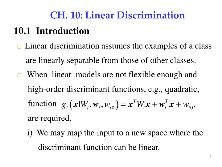
1. CH. 10: Linear Discrimination 10.1 Introduction Linear discrimination assumes the examples of a class are linearly separable from those of other classes. When linear models are not flexible enough and high-order discriminant functions, e.g., quadratic, ( 0 | , , i i i i g W w x w ) = + + T T i function x x w x , W w 0 i i are required. i) We may map the input to a new space where the discriminant function can be linear. 1

2. = = = x z ( ) x ( , x x ), ( , , , , ) z z z z z Example: 1 2 1 2 3 4 5 2 1 = = = = = = = = = ( ) x x ( ) x where , ( ) , , z x z x z x 1 1 1 2 z 2 2 3 3 2 2 = ( ) x ( ) x , z x 1 2 x x 4 4 5 5 ( ) ig x ii) Write as a linear combination of higher-order ( ) ( ) 1 j = K terms . i g = x w x j ij ( ): x ij Examples of basis functions ( ) 1 sin , log x ( ) x + , 1( ), 1( ), x c ax bx c 2 1 1 2 2 2 x m exp( ( ) / ), exp( c / ) c x m 1 2

3. Types of classification methods i. Class-based approach ii. Boundary-based approach Class-based approach = x ( ) x Choose if ( ) g max j C g i i j ( )' x : class discriminant function where j g s ( ( ( ) = ( ) x e.g., (prior probability) g p C j j ) ) = ( ) x x | (class likelihood) g p C j j = ( ) x x | (posterior density) g p C j j 3

4. Boundary-based approach x Choose ( )' : i g x if ( ) g 0, where C i boundary discriminant function i s e.g., This chapter concerns with boundary discriminant ( ) i x| ig functions which are assumed to be linear, ( ) 0 0 | , x w w x i i i i i g w w = + d = + T w x w 0 ij j i = 1 j 4

5. 10.3 Geometry of the Linear Discriminant 10.3.1 Two Classes ( ) x w x g = + T w 0 ( ) x if otherwise 0 C C g 1 Choose 2 x x Let and i.e., ( g be two points on the decision surface, 0, ( ) 0. g = = + = w x 1 2 = + x x ) 1 1 = T T T w x w x x is the normal of the hyperplane. w 0 ( ) 0 w w 1 0 2 0 1 2 5

6. w w + x x Rewrte = , r p x where : the projection p x of onto the hyperplane = w x ( ) x + = T 0 g w 0 w w = + = + + T T x w x w x ( ) g w r w 0 0 p = + + = + = T w x w x w w ( ) . w r g r r 0 p p = ( )/ x w . The distance of the hyperplane r g T w x w to the original is / . p 6

7. 10.3.2 Multiple Classes Discriminant functions: ( ) = + = C T i | , xw w x = , x 1, , g w w i K 0 0 i i i i 0 0 if otherwise ( ) i | , xw g w 0 i i i e.g., Linear classification Hyperplanes correspond to linear boundary discriminant functions H i g i 7

8. Pairwise Separation K(K-1)/2 discriminant functions ( ) = + T xw w x ij | , g w w 0 0 ij ij ij ij One for each pair of distinct classes x x 0 0 if if otherwise ( ) , ij i g C C i ( ) x = g ij j don't care x Choose if 0. C j i 8

9. 10.5 Parametric Discrimination For 2-calss case, let g ( ) ( ) = = x x | , then | 1 P C y P C y 1 2 0.5 y ( ) y Choose if or / 1 or log 1 ; otherwise . C y y C 1 2 ( ) / 1 0 y ( ) = log / 1 logit( ) y y y : logit transformation The inverse of logit( ), i.e., , is sigmoid. y = = y ( ) ( ) = x ( Let logit( ) log / 1 , / 1 , x y y y e y y ( ) = + = = + x x x x x 1 , (1 y ) , /(1 ), y e y e e y e e = + x 1/( 1) ) y e 9

10. If class densities are normal and share a common , ( ) ( 1 logit | is linear. x P C ) the ( P C ) | x ( ( ( ( ) ) x x x | | | P C P C P C ( ) ( ) = = 1 1 x logit | log log P C ( ) 1 1 1 C C 2 ( ( ) ) ) ) x x | | p p P C P C + 1 1 = log log 2 2 Bay's rule | P C i x ( ) ( ) ( ) = x | P C P C i i ( ( ) ) ( ( )( )( ) ) ( ( ) ) /2 1/2 d T 1 x x 2 exp 1/2 1 1 = log /2 1/2 d T 1 x x 2 exp 1/2 2 2 ( ( ) ) P C P C + 1 log 2 10

11. ( ( ) ) ( ( )( )( ) ) ( ( ) ) 1/2 /2 d T 1 x x 2 exp 1/2 1 1 log 1/2 /2 d T 1 x x 2 exp 1/2 2 2 ( ( )( )( ) ) ( ( ) ) T 1 x x exp 1/2 1 1 = log T 1 x x exp 1/2 2 2 ( ) ( ) ( ) ( ) T T 1 1 = x x x x /2 1 1 2 2 1 1 1 1 1 = + T T T T T x x x x 1 1 1 1 2 2 ( ) T 1 1 + = T T x /2 ( ) 2 2 1 2 1 1 T T ( )/2 1 1 2 2 11

12. ( ) T 1 = T x ( ) 1 2 1 1 1 1 + T T T T ( )/2 1 1 1 2 1 2 2 2 ( ) ( ) ( ) T T 1 1 = + T x ( ) /2 ) ( = 1 2 1 2 1 2 ( ( ) ) T 1 T x x logit | ( ) P C 1 1 2 ( ( ) ) P C P C ( ) ( ) T 1 + + = + T 1 w x /2 log w 1 2 1 2 0 2 ( ) 1 = w where , 1 2 ( ( ) ) P C P C 1 2 ( ) ( ) T 1 = + + 1 log w 0 1 2 1 2 2 12

13. Recall that the inverse of logit( ), i.e., , is g y y 1 = sigmoid of logit( ), . y y 1 exp( logit( )) + y ( ) ( ) P C x The inverse of logit | 1 1 1 w x ( ) = = x | P C ( ) ( ) 1 1 exp + x logit( | P C 1 exp + + T w 1 0 g During training, i) Estimate m m , , S 1 2 ( ) 1 = m m w ii) Replace , , with , , in S 1 2 1 2 1 2 ( ) ( ) T 1 = + and /2 w 0 1 2 1 2 13

14. During testing, ( ) ( ) if ( ) = = + T x x w x i) Compute logit | ; g P C w 1 0 ( ) x choose 0, or C g 1 ( ) = + T w x ii) Compute sigmoid ; y w 0 choose 10.6 Gradient Descent if 0.5 C y 1 Idea: Let E(w|X) be the error with parameters w on sample X. Look for w* = arg minwE(w | X). E E E w w T E w Gradient = , , ... , w 1 2 d 14

15. Gradient-descent: Starts from random w and updates w iteratively in the negative direction of gradient + E w = ; w i i + 1 t i t i = w w w i 10.7 Logistic Discrimination -- Model the ratio of class-conditional densities 15

16. 10.7.1 Two classes --Assume the log class-conditional density ratio is ( ( 2 | x p C ) ) ( P C x | p C linear, i.e., = + T o 1 x w log . w 0 ) | x ( ( ) ) x x x | | | P C P C P C ( ) ( ) = = 1 1 x logit | log log P C ( ) 1 1 1 2 ( ( ) ) ( ( ) ) x x | | p p C C P C P C = + = + T 1 1 w x log log w 0 Bayes' rule 2 2 ( ( ) ) P C P C = + o 1 where log w w 0 0 2 16

17. The inverse of is , which is ( ( 1 logit P C x ) ( ) ( ) ) P C x ) = x | 1| ( + T a sigmoid function of w x logit | P C w 1 0 1 w x ( ) = x i.e., | P C ( ) 1 1 exp + + T w 0 w and . w Learn = x x t t Given a sampe x , , X r 0 = = where 1 ( ), 0 ( ) r C r C 1 2 ( ) = = = Assume | ~ Bernoulli with r x 1| ) x x ( | , p P r P C 1 ) w X ( ( ) , = 1/ 1 exp + + T w x . p w ( l 0 )( ) ) ( t 1 r t = r w The sample likelihood: | 1 p p 0 t 17

18. = Define the error function as cross-entropy. E log l )( ) ( ) ( ) t 1 r t = = r w , | log log 1 E w X l p p 0 t ( ( ) = + t t log 1 log 1 r p r p t Using gradient-descent to minimize ( The update equations: ) w , | E w X 0 t t 1 1 E w r p r p ( ) = = t j 1 w p p x j t j ( ) + 1 = = t t j ( n j n j , 1,..., ; d = + . r p x j w w w j t E w ) + 1 = = t n n ; = + . w r p w w w 0 0 0 0 t 18 0

19. During testing: Given x, 1. Calculate p = + 1 w x ( ) + T 1 exp w 0 2. Choose otherwise if C 0.5; C p 1 . 2 10.7.2 Multiple Classes Consider K > 2 and take as the reference class. C K ( ( ) ) x x | C p p C = + T i o i w x i Assume linearity log g w 0 | K 19

20. ( ( ) ) ( ( ) ) ( ( ) ) ) ) x x x x | | C P C P C p p C P C P C = + i i i log log log | | Bayes' rule K K K ( ( P C P C ( ( K P C = + + = + T i o i T i w x w x i log w w 0 0 i K ) ) P C = + o i i where ) ) x log w w 0 0 i ( ( x | p C p C = + T i w x i exp w 0 i | K ( ( ) ) ( ) x x x | 1 | P C P C P C P C 1 1 K K = = + T i w x i K x exp w ( ) 0 i | | = = 1 1 i i K K 20

21. 1 ( ) = x | P C K 1 K + + T i w x 1 exp w 0 i = 1 i = 1 1 + x = = + = ( 1 1 (1 ) ) y x xy x y x 1 x y To treat all classes uniformly, write ( ) + T w x exp w ( ) 0 i = = x | : softmax function p P C i i K + T j w x exp w 0 j = 1 j w and . iw X = x r t t Learn Given a sampe , , 0 i = = x where 1 ( ); otherwise 0 r C r i i i 21

22. ( ) r x p Assume | ~ Multnomial where = p ( ( 0 , i i E w w 1, K = | ). x { }, i p ) ) | X ( p P C i i ( ) p t ir = w , | , l w X 0 i i i i t i = = t log log l r p i i i t i The update equations: E w ( ) + 1 = = t j t n j n j w x w w w ; = + . r p j j j t j E ( ) + 1 = = t j n j n j ; = + . w r p w w w 0 0 0 0 j j j w t 0 j 22

23. During testing: Given x, ( ) + T w x exp w 0 i = = , 1, , p i K 1. Calculate i K + T j w x exp w 0 j = 1 j = 2. Choose if max k . C p p i i k 23

24. 10.8 Discrimination by Regression 2-D case The regression model: ( ) 2 = + , where ~ t t 0, . r y N t t If using the sigmoid function. {0, 1}, can be constrained to lie in [0, 1] y r Assume a linear model, ( ) = + t T t w x sigmoid y w 0 ( ) = 1/ 1 exp + + T t w x w 0 24

25. 2 x : Assuming | ( , ), the smaple likelihood r N y ( ) 2 t t r y 1 ( ) = w , | exp l w X 0 2 2 2 t Maximize the log likelihood Minimize the sum of square error 1 , | 2 t Using gradient dexcent, ( ) 2 ( ) = t t w E w X r y 0 ( ) ( ) ( y y ) = t t t t t w x 1 , r y y y t ( ) = t t t t 1 . w r y 0 t 25

26. d - D (d > 2) case The regression model: ( ) 2 = + t t r y , where ~ 0, . N I K K Assume a linear model 1 w x ( ) = + = t i T i t w x sigmoid y w ( ) 0 i 1 exp + + T i t w 0 i The smaple likelihood 2 t t r y 1 ( ) = { , w } | i exp l w X 0 i i 1/2 2 2 /2 (2 ) d t 26

27. The error function 1 2 1 2 , ( ) 2 2 ( ) = = t t t t i { , w r y }| i E w X r y 0 i i i t t i = The update equations for 1, i K ( ) ( ) ( i y y ) = t t i t i t i t w x 1 , r y y y i i t ( ) = t t t i t i 1 . w r y 0 i i t 10.9 Learning to Rank Ranking is different from classification and regression and is sort of between the two 27

28. Let xu and xv be two instances (e.g., two movies). We prefer u to v implies that g(xu) > g(xv) where g(x) is a score function and is assumed to be linear g(x) = wTx. Ranking Error u v x x x ( ( ) ) ( ) g g g We prefer u to v implies that ( ) ( g g x , so error u v x ( ) g v u x ) is , if = | ) | )] u v u v w x x ( |{ , }) r r [ ( g ( E g + u v r r = T v u w x x u ( ) + v r r a+ is equal to a if and 0 otherwise. a where 0 28

29. w Using gradient descent, the update equation of E w w = = = v j u j x x ( ), 1, , j d j j Example: 29

30. Appendix: Conjugate Gradient Descent -- Drawback: can only minimize quadratic functions, e.g., ( ) 2 Advantage: guarantees to find the optimum solution in at most n iterations, where n is the size of matrix A. A-Conjugate Vectors: : n n A 1 = + T T w w w b w f A c Let square, symmetric, positive-definite matrix. Vectors are A-conjugate if ( ) ( ) 0, s s j i j = = { (0), (1), s s , ( s 1)} S n Ti A * If A = I (identity matrix), conjugacy = orthogonality. 30

31. The conjugate-direction method for finding the w to minimize f(w) is through ( w(0): an arbitrary initial vector, min ( ( ) 1 ( ) 2 1 ( ( ) ( )) ( ( ) 2 ( ( ) b Let ( ( ) ( )) w s f i d + = ( ) ( ), s i + w w 1) ( ) i i i = 0, , 1 where i n + ( )). s i ( ) i w f i is determined by = w b w A + T T w w Q f c + = + + ( )) s i T w s w s ( ( ) w A ( )) i f i i i i + + T w s ( )) i i c d + = 0 i 31

32. d d + = + T T ( ( ) w s w w s w ( )) i ( ) i ( ) i ( ) i ( ) i f i A A d d + + 2 T T T T w s s s b w b s ( ) i ( ) ( ) i ( ) ( ) i ( ) i A i A i = = + + T T T T s w w ( ) 2 s A i ( ) s ( ) s A i b s ( ) 0 ( ) i ( ) i ( ) i i A i ( ) ( ( ) i + T T T b s s w T w s ( ) i A i ( ) i ( )) i A i A i = 2 ( ) s ( ) s 32

33. s How to determine ( )? r i Define , which is in the steepest ( ) ( ) i A i = b w 1 2 = w b w A + T T ( ) w w . f c descent direction of ( ) = + ( ) w w b Q ( ) f A w = + = ( ) ( i r 1, , = 1 (A) s r s = Let ( ) ( ) i 1), i i b i n (0) s w (0) (0) A and multiply (A) by s(i-1)A, To determine ( ), i = + ( ) ( i T T s A i s s r s ( 1) ( ) ( 1) ( ( ) A 1)). i i i i = Ti A s s ( ) ( ) j 0, i j In order to be A-conjugate: 33

34. = + T T s A i r s A i s 0 ( 1) ( ) ( ) i ( 1) ( 1). i i T s A i r ( 1) A i s n ( ) generated by Eqs. (A) and (B) i , ( s = ( ) i (B) T s ( 1) ( 1) i (1), (2), s s 1) are A-conjugate. Desire that evaluating does not need to know A. ( ) i T r r r ( )( ( ) ( r i ( 1)) i i i = ( ) i Polak-Ribiere formula: T r 1) ( 1) i T r i r ( ) ( ) 1) ( r i i i = ( ) i Fletcher-Reeves formula: T r ( 1) 34

35. Summary: The conjugate-direction method minimizes 2 T T ( ) = + w w w p w 2 k d R + = ( ) ( ), i + = w w s Let ( w(0) is an arbitrary starting vector 1) ( ) i 0,1, , 1 i i i n ( ) w T R i + w ( )) i s ( ) i min ( ( ) i is determined by ( ) ( ( ) i + T T T p s s w s ( ) i ( )) i R i i R i = 2 ( ) s s ( ) = + ( ) ( i = s ( ) s r s r p ( )) w R ( ( 1) i ( ) i 1), ( ) 2( i i i i 1) R i T r ( ) i R i = = = s r p (0)), ( ) w R (0) (0) 2( i T s s ( 1) 35

36. Nonlinear Conjugate Gradient Algorithm Initialize w(0) by an appropriate process 36

37. Example: A comparison of the convergences of gradient descent (green) and conjugate gradient (red) for minimizing a quadratic function. Conjugate gradient converges in at most n steps where n is the size of the matrix of the system (here n=2). 37