Keynesian Economics: Effective Demand and Aggregate Supply

Keynesian economics emphasizes the importance of effective demand in determining income, output, and employment levels. Effective demand, as outlined by Keynes, is the equilibrium level of demand that is met by aggregate supply to maintain stable employment and output levels. It is influenced by factors such as the Aggregate Demand Function and Aggregate Supply Function, which play crucial roles in shaping economic outcomes.

• Keynesian economics
• Effective demand
• Aggregate supply
• Income analysis
• Economic equilibrium

harperrose Follow

Uploaded on Aug 10, 2024 | 0 Views

Download Presentation

Please find below an Image/Link to download the presentation.

The content on the website is provided AS IS for your information and personal use only. It may not be sold, licensed, or shared on other websites without obtaining consent from the author. Download presentation by click this link. If you encounter any issues during the download, it is possible that the publisher has removed the file from their server.

Presentation Transcript

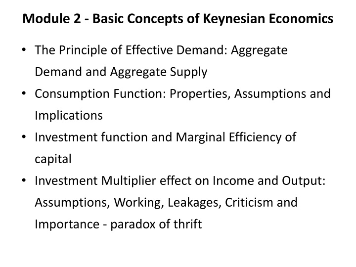
1. Module 2 - Basic Concepts of Keynesian Economics The Principle of Effective Demand: Aggregate Demand and Aggregate Supply Consumption Function: Properties, Assumptions and Implications Investment function and Marginal Efficiency of capital Investment Multiplier effect on Income and Output: Assumptions, Working, Leakages, Criticism and Importance - paradox of thrift

2. The Principle of Effective Demand Principle of effective demand is basic to Keynes analysis of income, output and employment. It is outlined in Keynes' path breaking book, "General theory on Employment, published in 1936. A fundamental principal is that as the real income increases, consumption will also increase but by an amount which is less than the increase in income. Therefore in order to have enough demand to sustain an increase in employment there must be an increase in real investment equal to the gap between income and consumption. Interest and Money",

3. Income Employment Effective Demand Aggregate Demand Function Aggregate Supply Function Consumption Expenditure Investment Expenditure Government Expenditure Rate of Interest Propensity to consume Marginal Efficiency of Capital Income Subjective Factors Objective Factors

4. Effective Demand The aggregate demand in a two sector economy consists of consumption demand and investment demand. At various level of employment and income, there are corresponding levels of demand, but all levels of demand are not effective only that level of demand is effective which is fully met by the aggregate supply so that the firms do not have tendency to increase or decrease the level of employment and output. Thus effective demand represents ' equilibrium level of employment.'

5. Determinants of Effective Demand According to Keynes, effective demand is determined by two factors 1. Aggregate Demand Function (ADF) 2. Aggregate Supply Function (ASF) 1. Aggregate Demand Function: It refers to the schedule of maximum sales proceeds which the firms expect to receive from the sale of output resulting from different levels of employment. Aggregate demand price is the amount of money which the firms expect to receive from the sale of output produced at a particular level of employment.

6. ADF ADF ADF O O Employment Employment The vertical intercept of ADF shows autonomous consumption (i.e. the level of expenditure at zero level of employment and output). Non-linear ADF shows that the propensity to consume diminishes along with the increase in employment and output. Linear curve shows constant marginal propensity to consume (MPC).

7. Determinants of Effective Demand 2. Aggregate Supply Function ASF refers to the schedule of minimum amount of sales proceeds or revenue, which the firms must get from the sale of output resulting from various levels of employment. In other words these are the minimum amounts which are considered just necessary to induce the firms to provide a certain level of employment. The ASF is also an increasing function of the level of employment. It is clear that the aggregate supply price depends on the cost of production.

8. ASF ASF ASF O O N Employment N Employment F F The ASF curve becomes vertical at the full level of 'NF'. Linear ASF represent homogenous cost function with constant returns. Non - linear ASF is more realistic as it represents diminishing returns in production function. Unlike the ADF curve which has positive Y - intercept. The ASF curve starts from the point of origin because for zero employment cost is also zero.

9. ASF ADF ASF ADF E O N N N N Employment F 1 2 ED is obtained at point E where ADF = ASF. The equil level of emp is given as 'ON'. To the left of the point 'E' or 'ON', ADF > ASF and emp will increase to 'ON'. At ON1 emp, ADF is higher than ASF and the firms are getting more than the required min. to continue in the production. the firms will increase the level of emp upto 'ON'. At 'ON2' level of emp, the ADF < ASP and the firms are getting less than the min price. They will reduce the level of emp and output..

10. Under-employment Equilibrium' In the diagram given above full employment is given as ONF , where as employment equilibrium is ON hence unemployment exist in the economy. There are two ways to attain full employment level (1) shifting the ADF upwards, (2) shifting the ASF downwards.

11. ASF ADF E 2 ASF ADF 2 E 1 ADF 1 O Employment N N 1 F The initial equilibrium level (effective demand) is at E1, but it shows under employment equilibrium. If ADF1 can be shifted to ADF2 in such a way that it passes through E2 so that full employment is obtained.

12. Consumption Function The consumption demand is a major component of aggregate demand. The level of consumption expenditure in an economy depends on the current level of income, current and expected price level, taste and preference, expected future income, etc. Keynes stated that in the short period consumption is a function of current real income. Symbolically, ( ( ) ) Y f C= = Consumption and income has a direct functional relationship.

13. Consumption Function According to Keynes, consumption function is governed by the Psychological Law of Consumption. It is stated as follows - "............. men are disposed, as a rule, and on the average, to increase their consumption as their income increases, but not by as much as the increase in their income.'' This means that the change in consumption ( C) is less than the change in income ( Y). Consumption function equation: = = + + C C cY 0 c C and 0 1

14. Attributes of Consumption Function Average propensity to consume (APC): The APC is the ratio of consumption expenditure to the corresponding level of income. . APC diminishes as income increases. Marginal propensity to consume: It is the ratio of change in consumption to change in income. . Following the psychological law of consumption, MPC lies between zero and one (0 < MPC < 1). C APC = = Y C = = MPC Y

15. Consumption and Saving Function Table MPC APC S MPS APS Y C ( C/ Y) (C/Y) (Y - C) ( S/ Y) (S/Y) 0 40 - - - 40 - - 100 120 0.8 1.2 - 20 0.2 0.2 200 200 0.8 1.0 0 0.2 0 300 280 0.8 0.93 20 0.2 0.7 400 360 0.8 0.9 40 0.2 0.1 500 440 0.8 0.88 60 0.2 0.12

16. Income Line Consumptio n & Saving = = + + C C cY Saving T S dissaving C 45 O Income Y

17. Explanation of the diagram The vertical intercept of the consumption function represents C or the autonomous consumption. The slope of the consumption function is given by the value of MPC. The 45 line is the income line. Every point on the income line shows C = Y. The consumption function intersects the income line at point T. Corresponding level of income is known as break - even level, because, C = Y and S = 0. Before the break - even level, saving is negative and afterwards saving is positive. The saving function is the counter part of the given consumption function. It passes through the x - axis at the income where C = Y.

18. Factors Affecting Consumption Function 1. Subjective factors: a) The motive of precaution b) Motive of foresight c) Motive of calculation d) The motive of improvement e) Motive of independence f) Motive of enterprises g) Motive of pride h) Motive of avarice

19. Factors Affecting Consumption Function 2. Objective Factors a) Windfall income b) Fiscal policy c) Changes in the rate of interest d) Distribution of income e) The level of holding of financial assets f) The level of wealth g) Expectation of price h) Level of income

20. Importance/Implications of the Consumption Function 1. It invalidates the Say's Law of market 2. It emphasises the necessity of investment 3. Need for state intervention 4. Turning point of trade cycles 5. Underemployment equilibrium

21. Investment function and Marginal Efficiency of capital Investment implies the addition to the capital stock i.e. plant and equipment. Therefore in employment theory investment refers to real investment and not the investment in second hand securities. Investment demand depends on two factors namely, 1. Marginal Efficiency of Capital (MEC or e) 2. Rate of Interest (i)

22. 1. Marginal Efficiency of capital The MEC refers to the profitability of the capital asset. It is the expected rate of return over cost or the expected profitability. MEC depends on two factors. i. Prospective yield (Q) ii. Supply price (P) As K. Kurihara states, MEC is the ratio between the prospective yield of additional asset and its supply price. Q e = = P

23. Marginal Efficiency of capital i. Prospective yield (Q): It is the expected annual net returns from production and sale of the output. Supply price is the cost of acquiring a new capital asset. The capital asset is durable and it gives net returns for a number of years, so we have to consider the sum of the annual net returns as the prospective yield. MEC refers to the rate at which the prospective yield from an additional capital asset is to be discounted, it is to be equal to its supply price. Q e 1 + + + + Q Q + + Q + + 1 1 e 1 e n = = + + + + + + + + SP ...... ( ( ) ) ( ( ) ) ( ( ) ) ( ( ) )n e 2 3 1 1 1

24. Marginal Efficiency of capital ii. Supply price of the capital asset: 'e' is the rate of discount of MEC. From the above equation it follows that MEC varies with the changes in the prospective yield and the supply price. Given the supply price, MEC will be higher, if the prospective yield (Q1, Q2, etc) is higher and vice- versa. Given the value of Q1, Q2, etc. MEC will be higher if supply price is lower.

25. Investment Demand Schedule Investment demand depends on the rate of interest and the MEC. Investment and rate of interest are inversely related, which means that at higher interest rate, investment demand will be lower and vice versa. Rate of Interest % p.a) (Rs. Crores) 10 10 Vol. of Investment MEC (% p.a.) 10 9 20 9 8 30 8 7 40 7 6 50 6

26. Supply Price and Demand Price The comparison between 'e' and 'i' is infact a comparison between the supply price of a capital asset and its demand price. Supply price is the cost of acquiring new asset. MEC is the rate which discounts the future net returns so that it is equal to the supply price. Demand price is the "sum of the expected future returns discounted at the rate of interest. 1 1 i 1 i 1 + + + + Q Q Q + + n = = + + + + + + DP ...... ( ( ) ) ( ( ) ) ( ( ) )n i 2 1 e > i DP > SP Investment will increase e = i DP = SP Investment will be in equilibrium e < i DP < SP Investment will fall

27. 2. Interest Elasticity of Investment Demand The slope of the investment demand curve depends on the interest elasticity of demand which again is related to how slowly or fast MEC falls to a given increase in investment. Investment demand is interestelastic , if MEC declines slowly to a increase in investment. This will mean that a greater increase in investment will be required to equate MEC with interest. If investment is interest elastic, the MEC schedule or investment demand curve is flatter. If investment is interestinelastic , investment demand curve will be steeper.

28. Factors Affecting Investment Function 1. Short run factors a) Nature of demand, prices and cost b) Propensity to consume c) Changes in liquid asset d) Business outlook 2. Long run factors: a) Population b) Techniques c) Development of backward areas

29. Investment Multiplier Investment Multiplier tells us about the changes in income for changes in the investment. The concept o Multiplier was developed by R.F. Kahn. With change in the investment here will be a change in the income, because the investment expenditure turns into income. There after the income induce the consumption to increase depending on the level of marginal propensity of consumption

30. Investment Multiplier This way an increase in the consumption expenditure creates incomes in the second round. The induced income again increases the consumption. This cycle repeats and an increase in the investment generates income several times more. This is called as the multiplier effect. Multiplier is the ratio of total change in income to the initial change in investment. Let K denote multiplier, then Y K I = =

31. Investment Multiplier The multiplier has a time lag. The multiplier works into the long run. Each year some income is added and consumption is generated. This may taper with time but it shall continue for ever, theoretically. This is called multiplier effect. Propensity of Consumption The intensity of consumption whether aggregate or additional is called propensity of consumption. Propensity of consumption can be measured in two ways. 1. Average propensity of consumption: APC is the ratio of consumption to Income.

32. Investment Multiplier C APC= Y 2. Marginal propensity of consumption: The MPC measures changes in consumption for changes in income. It is the measures of propensity of consume for an increment in C = MPC Y

33. Average Propensity to Consume Marginal Propensity to Consume consumption consumption Income Income C C APC= = MPC Y Y

34. Derivation of Multiplier Y = K I = + Y C S Y = = + K Y C I By substituting I with Y - C Y - C = + Y C I Y = I Y C Y = Dividing numerator and denominator with Y K Y - C Y Y Y By simplification = = K Y C Y Y 1 By factorization = K C - 1 Y 1 Since, C / Y = MPC K = - 1 MPC 1 K = Since, 1 MPC = MPS - 1 MPS

35. Working Process of the Multiplier I 100 Y 100 80 64 51.20 40.96 32.77 26.22 20.98 16.78 13.42 10.74 8.59 6.87 5.50 4.40 3.52 2.82 2.26 1.81 1.45 1.16 0.93 0.74 C 80 64 S 20 16 I Y 0.59 0.47 0.38 0.30 0.24 0.19 0.15 0.12 0.10 0.08 0.06 0.05 0.04 0.03 0.02 0.02 0.01 0.01 0.01 0.01 0.01 0.00 0.00 0.00 0.00 500 C 0.47 0.38 0.30 0.24 0.19 0.15 0.12 0.096 0.077 0.062 0.050 0.040 0.032 0.024 0.016 0.013 0.010 0.008 0.006 0.005 0.004 0.003 0.002 0.002 0.002 400 S 0.12 0.09 0.08 0.06 0.05 0.04 0.03 0.02 0.02 0.02 0.01 0.01 0.01 0.01 0.00 0.00 0.00 0.00 0.00 0.00 0.00 0.00 0.00 0.00 0.00 100 51.20 40.96 32.77 26.22 20.98 16.78 13.42 10.74 8.59 6.87 5.50 4.40 3.52 2.82 2.26 1.81 1.45 1.16 0.93 0.74 0.59 12.80 10.24 8.19 6.55 5.24 4.20 3.36 2.68 2.15 1.72 1.37 1.10 0.88 0.70 0.56 0.45 0.36 0.29 0.23 0.19 0.15 Total

36. = = Y AD + + C I I E 2 Aggregate Demand C+ I E 1 I C I C 45 0 Y Y National Income 1 2 Y Y 1 Y 2 I I

37. Leakages in the Multiplier Process Increase in saving or hoarding: When hoarding take place some amount of income disappears from the income flow this will reduce the value of multiplier (K). Purchase of old assets: The income recipients may buy old assets such as shares and securities from other people who may not increase their consumption or expenditure; this will reduce the value of K. Repayment of old debt: The income recipients may use the income to repay old debt instead of spending it on goods and services. Excess of import over exports: In this case there will be a net outflow of income which will reduce the value of K. Inflation: The rise in prices would require additional money expenditure even to buy the same quantity of goods and services. Hence the actual consumption demand will not increase. High taxes and corporate savings: High taxes and an increase in corporate savings will lead to a decline in consumption expenditure and the value of K. 1. 2. 3. 4. 5. 6.