Hidden Markov Models: Applications and Examples

Hidden Markov model
A
pplications
•
Speech recognition
•
Machine translation
•
Gene prediction
•
S
equences alignment
•
Time Series Analysis
•
Protein folding
•
…
Markov Model
•
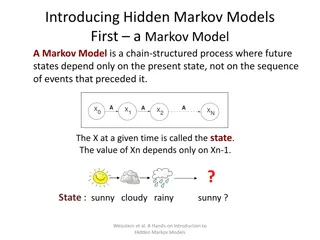
A system with states that obey the Markov assumption is called a
Markov Model
•
A sequence of states resulting from such a model is called a
Markov Chain.
An example
Hidden Markov model
•
A hidden Markov model (HMM) is a statistical Markov model in
which the system being modeled is assumed to be a Markov
process with unobserved (hidden) states.
Notice that only the observations y are visible, the states x are hidden to
the outside. This is where the name
Hidden Markov Models
comes from
Hidden Markov Models
•
Components:
–
Observed variables
•
Emitted symbols
–
Hidden variables
–
Relationships between them
•
Represented by a graph with transition probabilities
•
Goal:
Find the most likely explanation for
the observed variables
The occasionally dishonest casino
•
A casino uses a fair die most of the time, but
occasionally switches to a loaded one
–
Fair die: Prob(1) = Prob(2) = . . . = Prob(6) = 1/6
–
Loaded die: Prob(1) = Prob(2) = . . . = Prob(5) = 1/10,
Prob(6) = ½
–
These are the
emission
probabilities
•
Transition probabilities
–
Prob(Fair
–
Prob(
Loaded
Fair
) = 0.2
–
Transitions between states obey a Markov process
An HMM for the occasionally
dishonest casino
The occasionally dishonest casino
•
Known:
–
The structure of the model
–
The transition probabilities
•
Hidden: What the casino did
–
FFFFFLLLLLLLFFFF...
•
Observable: The series of die tosses
–
3415256664666153...
•
What we must infer:
–
When was a fair die used?
–
When was a loaded one used?
•
The answer is a sequence
FFFFFFFLLLLLLFFF...
Making the inference
•
Model assigns a probability to each explanation of the observation:
P(326|FFL)
= P(3|F)·P(F
·P(2|F)·P(F
·P(6|L)
= 1/6 · 0.99 · 1/6 · 0.01 · ½
•
Maximum Likelihood:
Determine which explanation is most likely
–
Find the path
most likely
to have produced the observed sequence
•
Total probability:
Determine probability that observed sequence was
produced by the HMM
–
Consider
all
paths that could have produced the observed sequence
Notation
•
x
is
the sequence of symbols emitted by model
–
x
i
is the symbol emitted at time
i
•
A
path
,
,
is a sequence of states
–
The
i
-
th state in
is
i
•
a
kr
is the probability of making a transition from state
k
to
state
r
:
•
e
k
(
b
)
is the probability that symbol
b
is emitted when in
state
k
A “pa
th
” of a sequence
x
1
x
2
x
3
x
L
2
1
K
2
The occasionally dishonest casino
The most probable path
The most likely path
*
satisfies
To find
*
,
consider all possible ways the last
symbol of
x
could have been emitted
Let
Then
The Viterbi Algorithm
•
Initialization
(
i
= 0
)
•
Recursion (
i
= 1, . . . ,
L
): For each state
k
•
Termination:
To find
*
, use trace-back, as in dynamic programming
Viterbi: Example
1
x
0
0
6
2
6
(
1/6
)
(1/2)
=
1/12
0
(
1/2
)
(1/2)
=
1/4
(
1/6
)
max{(1/12)
0.99,
(1/4)
0.2}
=
0.01375
(
1/10
)
max{(1/12)
0.01,
(1/4)
0.8}
=
0.02
B
F
L
0
0
(
1/6
)
max{0.01375
0.99,
0.02
0.2}
=
0.00226875
(
1/2
)
max{0.01375
0.01,
0.02
0.8}
=
0.08
Total probabilty
Many different paths can result in
observation
x
.
The probability that our model will emit
x
is
Total
Probability
If HMM models a family of objects, we
want total probability to peak at members
of the family
. (
Training
)
Total probabilty
Let
Then
Pr(
x
)
can be computed in the same way as
probability of most likely path.
and
The Forward Algorithm
•
Initialization (
i
= 0
)
•
Recursion (
i
= 1, . . . ,
L
): For each state
k
•
Termination:
Estimating the probabilities
(“training”)
•
Baum-Welch algorithm
–
Start with initial guess at transition probabilities
–
Refine guess to improve the total probability of the training data in
each step
•
May get stuck at local optimum
–
Special case of expectation-maximization (EM) algorithm
•
Viterbi training
–
Derive probable paths for training data using Viterbi algorithm
–
Re-estimate transition probabilities based on Viterbi path
–
Iterate until paths stop changing
Hidden Markov models (HMMs) are statistical models used in various fields such as speech recognition, machine translation, gene prediction, and more. They involve observable variables and hidden states, with the goal of finding the most likely explanation for the observations. This description covers the components of HMMs, including emitted symbols, transition probabilities, and the concept of hidden states. An example involving an occasionally dishonest casino illustrates the practical use of an HMM in inferring hidden information from observable data.

Download Presentation

Please find below an Image/Link to download the presentation.
The content on the website is provided AS IS for your information and personal use only. It may not be sold, licensed, or shared on other websites without obtaining consent from the author.If you encounter any issues during the download, it is possible that the publisher has removed the file from their server.
You are allowed to download the files provided on this website for personal or commercial use, subject to the condition that they are used lawfully. All files are the property of their respective owners.
The content on the website is provided AS IS for your information and personal use only. It may not be sold, licensed, or shared on other websites without obtaining consent from the author.
E N D
Presentation Transcript
Applications Speech recognition Machine translation Gene prediction Sequences alignment Time Series Analysis Protein folding
Markov Model A system with states that obey the Markov assumption is called a Markov Model A sequence of states resulting from such a model is called a Markov Chain.
Hidden Markov model A hidden Markov model (HMM) is a statistical Markov model in which the system being modeled is assumed to be a Markov process with unobserved (hidden) states.
Notice that only the observations y are visible, the states x are hidden to the outside. This is where the name Hidden Markov Models comes from
Hidden Markov Models Components: Observed variables Emitted symbols Hidden variables Relationships between them Represented by a graph with transition probabilities Goal: Find the most likely explanation for the observed variables
The occasionally dishonest casino A casino uses a fair die most of the time, but occasionally switches to a loaded one Fair die: Prob(1) = Prob(2) = . . . = Prob(6) = 1/6 Loaded die: Prob(1) = Prob(2) = . . . = Prob(5) = 1/10, Prob(6) = These are the emission probabilities Transition probabilities Prob(Fair Loaded) = 0.01 Prob(Loaded Fair) = 0.2 Transitions between states obey a Markov process
An HMM for the occasionally dishonest casino
The occasionally dishonest casino Known: The structure of the model The transition probabilities Hidden: What the casino did FFFFFLLLLLLLFFFF... Observable: The series of die tosses 3415256664666153... What we must infer: When was a fair die used? When was a loaded one used? The answer is a sequence FFFFFFFLLLLLLFFF...
Making the inference Model assigns a probability to each explanation of the observation: P(326|FFL) = P(3|F) P(F F) P(2|F) P(F L) P(6|L) = 1/6 0.99 1/6 0.01 Maximum Likelihood: Determine which explanation is most likely Find the path most likely to have produced the observed sequence Total probability: Determine probability that observed sequence was produced by the HMM Consider all paths that could have produced the observed sequence
Notation x isthe sequence of symbols emitted by model xi is the symbol emitted at time i A path, , is a sequence of states The i-th state in is i akr is the probability of making a transition from state k to state r: Pr( a i kr = = r | k ) = i 1 ek(b) is the probability that symbol b is emitted when in state k Pr( ) ( b e k = x b | k ) = = i i
A path of a sequence 1 1 1 1 1 2 2 2 2 2 2 0 0 K K K K K x1 x2 x3 xL L = i Pr( x , ) a e ( x ) a = i 0 i i i 1 1 + 1
The occasionally dishonest casino x x , x , x 6 , 2 , 6 = = 1 2 3 Pr( x , ) a e ( 6 ) a e ( 2 ) a e ( 6 ) ) 1 ( = 0 F F FF F FF F 1 1 1 FFF ) 1 ( = 5 . 0 . 0 99 . 0 99 = 6 6 6 . 0 00227 Pr( x , ) a e ( 6 ) a e ( 2 ) a e ( 6 ) ( 2 ) = LLL ( 2 ) = 0 L L LL L LL L 5 . 0 5 . 0 8 . 0 1 . 0 8 . 0 5 . 0 = . 0 008 = Pr( x , ) a e ( 6 ) a e ( 2 ) a e ( 6 ) a ( 3 ) = LFL ( 3 ) = 0 L L LF F FL L L 0 1 5 . 0 5 . 0 2 . 0 . 0 01 5 . 0 = 6 . 0 0000417
The most probable path The most likely path * satisfies arg = max Pr( x , ) * To find *, consider all possible ways the last symbol of x could have been emitted Let i v k = , , emit to 1 ( ) Prob. path of , , most likely i 1 x x such that k = i i Then ( v ) v ( i ) e ( x ) max ( i ) 1 a = r i k k rk r
The Viterbi Algorithm Initialization (i = 0) , 1 v v ( 0 ) ( 0 ) 0 for k 0 = = 0 k Recursion (i = 1, . . . , L): For each state k ( v ) v ( i ) e ( x ) max ( i ) 1 a = r i k k rk r Termination: ( v ) Pr( x , ) max k ( L ) a * = k k 0 To find *, use trace-back, as in dynamic programming
Viterbi: Example 2 0 x 6 0 6 0 B 1 (1/6) max{(1/12) 0.99, (1/4) 0.2} = 0.01375 (1/6) max{0.01375 0.99, 0.02 0.2} = 0.00226875 (1/6) (1/2) = 1/12 0 F (1/2) max{0.01375 0.01, 0.02 0.8} = 0.08 (1/10) max{(1/12) 0.01, (1/4) 0.8} = 0.02 (1/2) (1/2) = 1/4 0 L ( v ) v ( i ) e ( x ) max ( i ) 1 a = r i k k rk r
Total probabilty Many different paths can result in observation x. The probability that our model will emit x is Total Probability Pr( x ) Pr( x ) , = If HMM models a family of objects, we want total probability to peak at members of the family. (Training)
Total probabilty Pr(x) can be computed in the same way as probability of most likely path. Let f ( i ) observing of Prob. k x , , x = i 1 k assuming that = i Then r k f ( i ) e ( x ) f ( i ) 1 a = r i k k rk and Pr( x ) f ( L ) a = k k 0
The Forward Algorithm Initialization (i = 0) 0 f ( 0 ) , 1 f ( 0 ) 0 for k 0 = = k Recursion (i = 1, . . . , L): For each state k e i f ( ) ( r x ) f ( i ) 1 a = r i k k rk Termination: k Pr( x ) f ( L ) a = k k 0
Estimating the probabilities ( training ) Baum-Welch algorithm Start with initial guess at transition probabilities Refine guess to improve the total probability of the training data in each step May get stuck at local optimum Special case of expectation-maximization (EM) algorithm Viterbi training Derive probable paths for training data using Viterbi algorithm Re-estimate transition probabilities based on Viterbi path Iterate until paths stop changing