Introduction to Markov Decision Processes and Optimal Policies


Announcements
Assignments
HW7: Thu, 11/19, 11:59 pm
Schedule change
Friday: Lecture in all three recitation slots
Monday: Recitation in both lecture slots
Final exam scheduled
Study groups

Introduction to
Machine Learning
Markov Decision
Processes


Instructor: Pat Virtue
Plan
Last time
Applications of sequential decision making (and Gridworld
)
Minimax and expectimax trees
MDP setup
Markov Decision Processes
An MDP is defined by:
A
set of states s
S
A
set of actions a
A
A
transition function T(s, a, s
’)
Probability that a from s leads to s’, i.e., P(s
’| s, a)
Also called the model or the dynamics
A
reward function R(s, a, s
’)
Sometimes just R(s) or R(s
’)
A
start state
Maybe a
terminal state
MDPs are non-deterministic search problems
One way to solve them is with expectimax search
We’
ll have a new tool soon
[Demo – gridworld manual intro (L8D1)]
Slide: ai.berkeley.edu
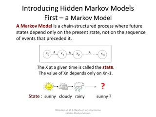
What is Markov about MDPs?
“Markov” generally means that given the present state, the future
and the past are independent
For Markov decision processes,
“Markov” means action outcomes
depend only on the current state
Andrey Markov
(1856-1922)
Slide: ai.berkeley.edu
Policies
Optimal policy when R(s, a, s
’) = -0.03
for all non-terminals s
We don’t just want an optimal
plan
, or sequence
of actions, from start to a goal
For MDPs, we want an optimal
policy
*: S → A
A policy gives an action for each state
An optimal policy is one that maximizes
expected utility if followed
Expectimax didn’t compute entire policies
It computed the action for a single state only
Slide: ai.berkeley.edu
Plan
Optimal Policies
R(s) = -2.0
R(s) = -0.4
R(s) = -0.03
R(s) = -0.01
Slide: ai.berkeley.edu
Example: Racing
Slide: ai.berkeley.edu
Example: Racing
A robot car wants to travel far, quickly
Three states:
Cool
,
Warm
, Overheated
Two actions:
Slow
,
Fast
Going faster gets double reward
1.0
Slow
(R=1)
Fast
(R=2)
0.5
0.5
0.5
Fast
(R=-10)
Slow
(R=1)
1.0
0.5
Slide: ai.berkeley.edu
Racing Search Tree
Slide: ai.berkeley.edu
MDP Search Trees
Each MDP state projects an expectimax-like search tree
a
s
s
’
s, a
(s,a,s
’
) called a
transition
T(s,a,s
’
) = P(s
’
|s,a)
R(s,a,s
’
)
s,a,s
’
s is a
state
(s, a) is a
q-
state
Slide: ai.berkeley.edu
Recursive Expectimax
a
s
s
’
s, a
s,a,s
’
Recursive Expectimax
a
s
s
’
s, a
s,a,s
’
Simple Deterministic Example
Actions: B, C, D: East, West
Actions: A, E:
Exit
Transitions: deterministic
Rewards only for transitioning to terminal state
T (Terminal)
R(A, Exit, T) = 10
R(A, Exit, T) = 1
Simple Deterministic Example
T (Terminal)
R(A, Exit, T) = 10
R(A, Exit, T) = 1
Actions: B, C, D: East, West
Actions: A, E: Exit
Transitions: deterministic
Rewards only for transitioning to terminal state
Utilities of Sequences
Slide: ai.berkeley.edu
Utilities of Sequences
What preferences should an agent have over reward sequences?
More or less?
Now or later?
[1, 2, 2]
[2, 3, 4]
or
[0, 0, 1]
[1, 0, 0]
or
Slide: ai.berkeley.edu
Discounting
It’s reasonable to maximize the sum of rewards
It’s also reasonable to prefer rewards now to rewards later
One solution: values of rewards decay exponentially
Worth Now
Worth Next Step
Worth In Two Steps
Slide: ai.berkeley.edu
Discounting
How to discount?
Each time we descend a level, we
multiply in the discount once
Why discount?
Sooner rewards probably do have
higher utility than later rewards
Also helps our algorithms converge
Slide: ai.berkeley.edu
Discounting
Slide: ai.berkeley.edu
T (Terminal)
R(A, Exit, T) = 10
R(A, Exit, T) = 1
Infinite Utilities?!
Problem: What if the game lasts forever? Do we get infinite rewards?
Solutions:
Finite horizon: (similar to depth-limited search)
Terminate episodes after a fixed T steps (e.g. life)
Gives nonstationary policies (
depends on time left)
Discounting: use 0 < < 1
Smaller means smaller
“
horizon
”
– shorter term focus
Absorbing state: guarantee that for every policy, a terminal state will eventually be
reached (like
“
overheated
”
for racing)
Slide: ai.berkeley.edu
Solving MDPs
Slide: ai.berkeley.edu
Value Iteration
Slide: ai.berkeley.edu
Value Iteration
Start with V
0
(s) = 0: no time steps left means an expected reward sum of zero
Given vector of V
k
(s) values, do one ply of expectimax from each state:
Repeat until convergence
Slide: ai.berkeley.edu
k=0
Noise = 0.2
Discount = 0.9
Living reward = 0
Slide: ai.berkeley.edu
k=1
Noise = 0.2
Discount = 0.9
Living reward = 0
Slide: ai.berkeley.edu
k=2
Noise = 0.2
Discount = 0.9
Living reward = 0
Slide: ai.berkeley.edu
k=3
Noise = 0.2
Discount = 0.9
Living reward = 0
Slide: ai.berkeley.edu
k=4
Noise = 0.2
Discount = 0.9
Living reward = 0
Slide: ai.berkeley.edu
k=5
Noise = 0.2
Discount = 0.9
Living reward = 0
Slide: ai.berkeley.edu
k=6
Noise = 0.2
Discount = 0.9
Living reward = 0
Slide: ai.berkeley.edu
k=7
Noise = 0.2
Discount = 0.9
Living reward = 0
Slide: ai.berkeley.edu
k=8
Noise = 0.2
Discount = 0.9
Living reward = 0
Slide: ai.berkeley.edu
k=9
Noise = 0.2
Discount = 0.9
Living reward = 0
Slide: ai.berkeley.edu
k=10
Noise = 0.2
Discount = 0.9
Living reward = 0
Slide: ai.berkeley.edu
k=11
Noise = 0.2
Discount = 0.9
Living reward = 0
Slide: ai.berkeley.edu
k=12
Noise = 0.2
Discount = 0.9
Living reward = 0
Slide: ai.berkeley.edu
k=100
Noise = 0.2
Discount = 0.9
Living reward = 0
Slide: ai.berkeley.edu
Exercise
As we moved from k=1 to k=2 to k=3, how did we get these specific
values for s=(2,2)?
2
1
0
2
1
0
3
Racing Tree Example
Slide: ai.berkeley.edu
Example: Value Iteration
0 0 0
2 1 0
3.5 2.5 0
1.0
Slow
(R=1)
Fast
(R=2)
0.5
0.5
0.5
Fast
(R=-10)
Slow
(R=1)
1.0
0.5
Slide: ai.berkeley.edu
Convergence
How do we know the V
k
vectors are going to converge?
Case 1: If the tree has maximum depth M, then V
M
holds
the actual untruncated values
Case 2: If the discount is less than 1
Sketch: For any state V
k
and V
k+1
can be viewed as depth k+1
expectimax results in nearly identical search trees
The difference is that on the bottom layer, V
k+1
has actual
rewards while V
k
has zeros
That last layer is at best all R
MAX
It is at worst R
MIN
But everything is discounted by
γ
k
that far out
So V
k
and V
k+1
are at most
γ
k
max|R| different
So as k increases, the values converge
Slide: ai.berkeley.edu
Value Iteration
Start with V
0
(s) = 0: no time steps left means an expected reward sum of zero
Given vector of V
k
(s) values, do one ply of expectimax from each state:
Repeat until convergence
Slide: ai.berkeley.edu
Piazza Poll 1
Piazza Poll 1
Value Iteration
Start with V
0
(s) = 0: no time steps left means an expected reward sum of zero
Given vector of V
k
(s) values, do one ply of expectimax from each state:
Repeat until convergence
Complexity of each iteration: O(S
2
A)
Theorem: will converge to unique optimal values
Basic idea: approximations get refined towards optimal values
Policy may converge long before values do
Slide: ai.berkeley.edu
Optimal Quantities
The value (utility) of a state s:
V
*
(s) = expected utility starting in s and
acting optimally
The value (utility) of a q-state (s,a):
Q
*
(s,a) = expected utility starting out
having taken action a from state s and
(thereafter) acting optimally
The optimal policy:
*
(s) = optimal action from state s
a
s
s
’
s, a
(s,a,s’) is a
transition
s,a,s’
s is a
state
(s, a) is a
q-state
[Demo – gridworld values (L8D4)]
Snapshot of Demo – Gridworld V Values
Noise = 0.2
Discount = 0.9
Living reward = 0
Slide: ai.berkeley.edu
Snapshot of Demo – Gridworld Q Values
Noise = 0.2
Discount = 0.9
Living reward = 0
Slide: ai.berkeley.edu
Values of States
Fundamental operation: compute the (expectimax) value of a state
Expected utility under optimal action
Average sum of (discounted) rewards
This is just what expectimax computed!
Recursive definition of value:
Slide: ai.berkeley.edu
The Bellman Equations
How to be optimal:
Step 1: Take correct first action
Step 2: Keep being optimal
Slide: ai.berkeley.edu
The Bellman Equations
Definition of
“optimal utility” via expectimax recurrence
gives a simple one-step lookahead relationship amongst
optimal utility values
Slide: ai.berkeley.edu
The Bellman Equations
Definition of
“optimal utility” via expectimax recurrence
gives a simple one-step lookahead relationship amongst
optimal utility values
Slide: ai.berkeley.edu
The Bellman Equations
Definition of
“optimal utility” via expectimax recurrence
gives a simple one-step lookahead relationship amongst
optimal utility values
Slide: ai.berkeley.edu
The Bellman Equations
Definition of
“optimal utility” via expectimax recurrence
gives a simple one-step lookahead relationship amongst
optimal utility values
These are the Bellman equations, and they characterize
optimal values in a way we’ll use over and over
Slide: ai.berkeley.edu
MDP Notation
Standard expectimax:
Bellman equations:
Value iteration:
MDP Notation
Standard expectimax:
Bellman equations:
Value iteration:
Synchronous vs Asynchronous Value Iteration
asynchronous
updates
: compute
and update V(s) for
each state one at a
time
synchronous
updates
: compute all
the fresh values of
V(s) from all the stale
values of V(s), then
update V(s) with
fresh values
Solved MDP! Now what?
What are we going to do with these values??
Explore the world of Markov Decision Processes (MDPs) and optimal policies in Machine Learning. Uncover the concepts of states, actions, transition functions, rewards, and policies. Learn about the significance of Markov property in MDPs, Andrey Markov's contribution, and how to find optimal policies using techniques like value iteration and Bellman equations.

Download Presentation

Please find below an Image/Link to download the presentation.
The content on the website is provided AS IS for your information and personal use only. It may not be sold, licensed, or shared on other websites without obtaining consent from the author. Download presentation by click this link. If you encounter any issues during the download, it is possible that the publisher has removed the file from their server.
E N D
Presentation Transcript
Announcements Assignments HW7: Thu, 11/19, 11:59 pm Schedule change Friday: Lecture in all three recitation slots Monday: Recitation in both lecture slots Final exam scheduled Study groups
Introduction to Machine Learning Markov Decision Processes Instructor: Pat Virtue
Plan Last time Applications of sequential decision making (and Gridworld ) Minimax and expectimax trees MDP setup
Markov Decision Processes An MDP is defined by: A set of states s S A set of actions a A A transition function T(s, a, s ) Probability that a from s leads to s , i.e., P(s | s, a) Also called the model or the dynamics A reward function R(s, a, s ) Sometimes just R(s) or R(s ) A start state Maybe a terminal state MDPs are non-deterministic search problems One way to solve them is with expectimax search We ll have a new tool soon Slide: ai.berkeley.edu [Demo gridworld manual intro (L8D1)]
What is Markov about MDPs? Markov generally means that given the present state, the future and the past are independent For Markov decision processes, Markov means action outcomes depend only on the current state Andrey Markov (1856-1922) Slide: ai.berkeley.edu
Policies We don t just want an optimal plan, or sequence of actions, from start to a goal For MDPs, we want an optimal policy *: S A A policy gives an action for each state An optimal policy is one that maximizes expected utility if followed Expectimax didn t compute entire policies It computed the action for a single state only Optimal policy when R(s, a, s ) = -0.03 for all non-terminals s Slide: ai.berkeley.edu
Plan Last time MDP setup Today Rewards and Discounting Finding optimal policies: Value iteration and Bellman equations How to use optimal policies Next time What happens if we don t have ? ? ?,? and ?(?,?,? )??
Optimal Policies R(s) = -0.03 R(s) = -0.01 R(s) = -0.4 R(s) = -2.0 Slide: ai.berkeley.edu
Example: Racing Slide: ai.berkeley.edu
Example: Racing A robot car wants to travel far, quickly Three states: Cool, Warm, Overheated 1.0 Two actions: Slow, Fast Fast +1 0.5 0.5 Going faster gets double reward 1.0 (R=-10) Slow Fast Slow (R=1) -10 +1 0.5 0.5 Slow Warm Slow (R=1) +2 Fast Fast (R=2) 0.5 0.5 0.5 Cool Overheated +1 1.0 1.0 +2 0.5 Slide: ai.berkeley.edu
Racing Search Tree Slide: ai.berkeley.edu
MDP Search Trees Each MDP state projects an expectimax-like search tree s is a state s a (s, a) is a q- state s, a (s,a,s ) called a transition T(s,a,s ) = P(s |s,a) s,a,s R(s,a,s ) s Slide: ai.berkeley.edu
Recursive Expectimax ? ? ?,?) ?(? ) ? ? = max ? s ? a s, a s,a,s s
Recursive Expectimax ? ? ?,?) ? ?,?,? + ? ? ? ? = max ? s ? a s, a s,a,s s
T (Terminal) Simple Deterministic Example Actions: B, C, D: East, West Actions: A, E: Exit Transitions: deterministic Rewards only for transitioning to terminal state ? ?,?,? + ? ? R(A, Exit, T) = 10 R(A, Exit, T) = 1 A B C D E ? ? = max ?
T (Terminal) Simple Deterministic Example Actions: B, C, D: East, West Actions: A, E: Exit Transitions: deterministic Rewards only for transitioning to terminal state R(A, Exit, T) = 10 R(A, Exit, T) = 1 A B C D E ? ?,?,? + ??? ??+1? = max ?
Utilities of Sequences Slide: ai.berkeley.edu
Utilities of Sequences What preferences should an agent have over reward sequences? More or less? [1, 2, 2] or [2, 3, 4] Now or later? [0, 0, 1] or [1, 0, 0] Slide: ai.berkeley.edu
Discounting It s reasonable to maximize the sum of rewards It s also reasonable to prefer rewards now to rewards later One solution: values of rewards decay exponentially Worth Now Worth Next Step Worth In Two Steps Slide: ai.berkeley.edu
Discounting How to discount? Each time we descend a level, we multiply in the discount once Why discount? Sooner rewards probably do have higher utility than later rewards Also helps our algorithms converge Slide: ai.berkeley.edu
T (Terminal) Discounting Actions: B, C, D: East, West Actions: A, E: Exit Transitions: deterministic Rewards only for transitioning to terminal state ??+1? = max ? For = 1, what is the optimal policy? R(A, Exit, T) = 10 R(A, Exit, T) = 1 A B C D E ? ?,?,? + ? ??? For = 0.1, what is the optimal policy? For which are West and East equally good when in state d? Slide: ai.berkeley.edu
Infinite Utilities?! Problem: What if the game lasts forever? Do we get infinite rewards? Solutions: Finite horizon: (similar to depth-limited search) Terminate episodes after a fixed T steps (e.g. life) Gives nonstationary policies ( depends on time left) Discounting: use 0 < < 1 Smaller means smaller horizon shorter term focus Absorbing state: guarantee that for every policy, a terminal state will eventually be reached (like overheated for racing) Slide: ai.berkeley.edu
Solving MDPs Slide: ai.berkeley.edu
Value Iteration Slide: ai.berkeley.edu
Value Iteration Start with V0(s) = 0: no time steps left means an expected reward sum of zero Given vector of Vk(s) values, do one ply of expectimax from each state: Vk+1(s) a s, a s,a,s Repeat until convergence Vk(s ) Slide: ai.berkeley.edu
k=0 Noise = 0.2 Discount = 0.9 Living reward = 0 Slide: ai.berkeley.edu
k=1 Noise = 0.2 Discount = 0.9 Living reward = 0 Slide: ai.berkeley.edu
k=2 Noise = 0.2 Discount = 0.9 Living reward = 0 Slide: ai.berkeley.edu
k=3 Noise = 0.2 Discount = 0.9 Living reward = 0 Slide: ai.berkeley.edu
k=4 Noise = 0.2 Discount = 0.9 Living reward = 0 Slide: ai.berkeley.edu
k=5 Noise = 0.2 Discount = 0.9 Living reward = 0 Slide: ai.berkeley.edu
k=6 Noise = 0.2 Discount = 0.9 Living reward = 0 Slide: ai.berkeley.edu
k=7 Noise = 0.2 Discount = 0.9 Living reward = 0 Slide: ai.berkeley.edu
k=8 Noise = 0.2 Discount = 0.9 Living reward = 0 Slide: ai.berkeley.edu
k=9 Noise = 0.2 Discount = 0.9 Living reward = 0 Slide: ai.berkeley.edu
k=10 Noise = 0.2 Discount = 0.9 Living reward = 0 Slide: ai.berkeley.edu
k=11 Noise = 0.2 Discount = 0.9 Living reward = 0 Slide: ai.berkeley.edu
k=12 Noise = 0.2 Discount = 0.9 Living reward = 0 Slide: ai.berkeley.edu
k=100 Noise = 0.2 Discount = 0.9 Living reward = 0 Slide: ai.berkeley.edu
Exercise As we moved from k=1 to k=2 to k=3, how did we get these specific values for s=(2,2)? 0 1 2 3 2 1 0
Racing Tree Example Slide: ai.berkeley.edu
Example: Value Iteration Fast (R=-10) 1.0 0.5 Slow (R=1) 0.5 Slow (R=1) 3.5 2.5 0 Fast (R=2) 0.5 1.0 2 1 0 0.5 Assume no discount! ? = 1 0 0 0 Slide: ai.berkeley.edu
Value Iteration Start with V0(s) = 0: no time steps left means an expected reward sum of zero Given vector of Vk(s) values, do one ply of expectimax from each state: Vk+1(s) a s, a s,a,s Repeat until convergence Vk(s ) Slide: ai.berkeley.edu
Piazza Poll 1 What is the complexity of each iteration in Value Iteration? S -- set of states; A -- set of actions Vk+1(s) I: ?(|?||?|) II: ?( ?2|?|) III: ?(|?| ?2) IV: ?( ?2?2) V: ?( ?2) a s, a s,a,s Vk(s )
Piazza Poll 1 What is the complexity of each iteration in Value Iteration? S -- set of states; A -- set of actions Vk+1(s) I: ?(|?||?|) II: ?( ?2|?|) III: ?(|?| ?2) IV: ?( ?2?2) V: ?( ?2) a s, a s,a,s Vk(s )
Value Iteration Start with V0(s) = 0: no time steps left means an expected reward sum of zero Given vector of Vk(s) values, do one ply of expectimax from each state: Vk+1(s) a s, a s,a,s Repeat until convergence Vk(s ) Slide: ai.berkeley.edu Complexity of each iteration: O(S2A) Theorem: will converge to unique optimal values Basic idea: approximations get refined towards optimal values Policy may converge long before values do
Optimal Quantities The value (utility) of a state s: V*(s) = expected utility starting in s and acting optimally s is a state s a (s, a) is a q-state The value (utility) of a q-state (s,a): Q*(s,a) = expected utility starting out having taken action a from state s and (thereafter) acting optimally s, a s,a,s (s,a,s ) is a transition s The optimal policy: *(s) = optimal action from state s [Demo gridworld values (L8D4)]
Snapshot of Demo Gridworld V Values Noise = 0.2 Discount = 0.9 Living reward = 0 Slide: ai.berkeley.edu
Snapshot of Demo Gridworld Q Values Noise = 0.2 Discount = 0.9 Living reward = 0 Slide: ai.berkeley.edu
Values of States Fundamental operation: compute the (expectimax) value of a state Expected utility under optimal action Average sum of (discounted) rewards This is just what expectimax computed! s a Recursive definition of value: s, a s,a,s s Slide: ai.berkeley.edu


")
")


")