Flow Distribution & Piezometric Head Calculation for Piping System
Determine flow distribution and piezometric heads at junction J using Newton-Raphson method for a piping system with specified dimensions, friction factors, and power input. The iterative calculations involve nodal discharges and head loss functions to optimize flow distribution in the system. Key variables such as pipe lengths, diameters, and initial discharges are utilized to converge towards the final solution.

Download Presentation

Please find below an Image/Link to download the presentation.
The content on the website is provided AS IS for your information and personal use only. It may not be sold, licensed, or shared on other websites without obtaining consent from the author. Download presentation by click this link. If you encounter any issues during the download, it is possible that the publisher has removed the file from their server.
E N D
Presentation Transcript
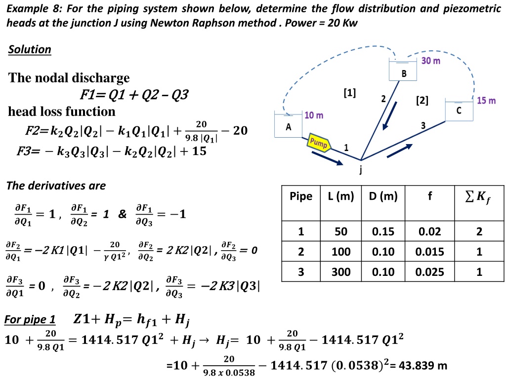
Example 8: For the piping system shown below, determine the flow distribution and piezometric heads at the junction J using Newton Raphson method . Power = 20 Kw Solution The nodal discharge F F1 1= Q head loss function F F2 2= = ?????? ??????+ F F3 3= = ?????? ??????+ ?? [1] = Q1 1 + Q + Q2 2 Q Q3 3 [2] ?? ?.? ?? ?? The derivatives are ?? Pipe L (m) D (m) f ??? ???= ? , ??? ??? = 1 & ??? ???= ? 1 50 0.15 0.02 2 ??? ???= = 2 2 K K1 1 ?? ?? ??? ??? = 2 2 K K2 2 ?? , ??? ? ???, ???= = 0 2 100 0.10 0.015 1 3 300 0.10 0.025 1 ??? ??? = ? , ??? ??? = 2 2 K K2 2 ?? , ??? ???= 2 2 K K3 3 ?? For pipe 1 ??+ ??= ???+ ?? ?? + ?? ?? ?.? ??= ????.??? ??? ?.? ?? ????.??? ??? + ?? ??= ?? + =?? + ?? ?.? ? ?.???? ????.??? (?.????)?= 43.839 m
Solving the above equations such that : ?? ?? ? ??? ??? ??? ??? ??? ??? ??? ??? ??? ??? ??? ??? ??? ??? ??? ??? ??? ??? ?? = ?? ?? ?? ?1 ?1 1 1 1 1 0 ?? 2 2 K K1 1 ?? 2 2 K K2 2 ?? ?2 = ?2 ? ??? 0 2 2 K K2 2 ?? 2 2 K K3 3 ?? ?3 ?3 Assuming initial pipe discharge in pipes, Q1 = 0.05 , Q2 = 0.05 & Q3 = 0.1 . ?? ? ? ? ? ? ? ???.?? ? ????.?? ????.?? ?? = ??.?? ?????.?? ???.?? ??
All details of the solution are explained in the following table Newton Raphson Method Pump Position Example 8 Pipoe no. L f D Ri Ki Pipe 1 Pipe 2 Pipe 3 65 107 304 0.02 0.015 0.025 0.15 0.1 0.1 0 0 0 1414.5174 13224.429 62796.412 Matrix of Derivatives Inverse Matrix Iteration 1 Q1 Q2 Q3 Qnew 0.045 0.008 0.053 Q -0.0052 -0.0418 -0.0470 F1 F2 F3 0.0500 0.0500 0.1000 0.00 50.34 -646.03 1.00 -957.78 0.00 1.00 1322.44 -1322.44 -12559.28 -1.00 0.00 0.5554 -0.0005 0.4022 0.0004 -0.0424 0.0000 0.0000 0.0000 -0.0001 Matrix of Derivatives Inverse Matrix Iteration 2 Q1 Q2 Q3 Qnew 0.058 -0.029 0.030 Q 0.0137 -0.0368 -0.0232 F1 F2 F3 0.0448 0.0082 0.0530 0.00 23.60 -162.06 1.00 -1143.58 0.00 1.00 216.01 -216.01 -1.00 0.00 -6652.25 0.1547 -0.0007 0.8188 0.0007 -0.0266 0.0000 0.0000 -0.0001 -0.0001
Matrix of Derivatives Inverse Matrix Iteration 3 Q1 Q2 Q3 Qnew 0.054 -0.032 0.022 Q -0.0042 -0.0032 -0.0073 F1 F2 F3 0.0585 -0.0287 0.0298 0.00 -0.81 -29.90 1.00 -762.26 0.00 1.00 758.39 -758.39 -1.00 0.00 -3742.91 0.4527 -0.0007 0.4551 0.0006 -0.0922 -0.0001 -0.0001 -0.0001 -0.0002 Matrix of Derivatives Inverse Matrix Iteration 4 Q1 Q2 Q3 Qnew 0.054 -0.032 0.021 Q -0.0005 -0.0005 -0.0010 F1 F2 F3 0.0543 -0.0318 0.0225 0.00 0.04 -3.26 1.00 -846.28 0.00 1.00 841.75 -841.75 -1.00 0.00 -2819.83 0.4337 -0.0007 0.4361 0.0005 -0.1302 -0.0002 -0.0002 -0.0002 -0.0003 Matrix of Derivatives Inverse Matrix Iteration 5 Q1 Q2 Q3 Qnew 0.054 -0.032 0.021 Q 0.0000 0.0000 0.0000 F1 F2 F3 0.0538 -0.0323 0.0215 0.00 0.00 -0.06 1.00 -857.25 0.00 1.00 855.60 -855.60 -1.00 0.00 -2694.22 0.4310 -0.0007 0.4318 0.0005 -0.1371 -0.0002 -0.0002 -0.0002 -0.0003 Matrix of Derivatives Inverse Matrix Iteration 6 Q1 Q2 Q3 Qnew 0.054 -0.032 0.021 Q 0.0000 0.0000 0.0000 F1 F2 F3 0.0538 -0.0324 0.0214 0.00 0.00 0.00 1.00 -857.49 0.00 1.00 855.84 -855.84 -1.00 0.00 -2691.82 0.4309 -0.0007 0.4318 0.0005 -0.1373 -0.0002 -0.0002 -0.0002 -0.0003 Note that for Q2= - 0.0324, it means that the flow must be in the opposite direction
Note that : Another assumption If the direction of flow was assumed as follows : Then the solution will take the following form: Solution The nodal discharge F F1 1= Q head loss function F F2 2= = - - ?????? ??????+ F F3 3= = ??????+ ??????+ ?? [1] [2] = Q1 1 - - Q Q2 2 Q Q3 3 ?? ?.? ?? ?? The derivatives are ?? Pipe L (m) D (m) f ??? ???= ? , ??? ??? = -1 & ??? ???= ? 1 50 0.15 0.02 2 ??? ???= = 2 2 K K1 1 ?? ?? ??? ??? = -2 2 K K2 2 ?? , ??? ? ???, ???= = 0 2 100 0.10 0.015 1 3 300 0.10 0.025 1 ??? ??? = ? , ??? ??? = +2 2 K K2 2 ?? , ??? ???= 2 2 K K3 3 ?? For pipe 1 ??+ ??= ???+ ?? ?? + ?? ?? ?.? ??= ????.??? ??? ?.? ?? ????.??? ??? + ?? ??= ?? + =?? + ?? ?.? ? ?.???? ????.??? (?.????)?= 43.839 m
Solving the above equations such that : ?? ?? ? ??? ??? ??? ??? ??? ??? ??? ??? ??? ??? ??? ??? ??? ??? ??? ??? ??? ??? ?? = ?? ?? ?? ?1 ?1 1 1 1 1 0 ?? 2 2 K K1 1 ?? 2 2 K K2 2 ?? ?2 = ?2 ? ??? 0 + +2 2 K K2 2 ?? 2 2 K K3 3 ?? ?3 ?3 Assuming initial pipe discharge in pipes, Q1 = 0.1 , Q2 = 0.06 & Q3 = 0.04 . ?? ? ? ? ? ? ? ???.?? ? ????.?? ????.?? ?? = ??.?? ????.?? ??.?? ??
All details of the solution are explained in the following table Newton Raphson Method Pump Position Example 8 Pipoe no. L f D Ri Ki Another Assumption Pipe 1 Pipe 2 Pipe 3 65 107 304 0.02 0.015 0.025 0.15 0.1 0.1 0 0 0 1414.5174 13224.429 62796.412 Matrix of Derivatives Inverse Matrix Iteration 1 Q1 Q2 Q3 Qnew 0.058 0.034 0.024 Q -0.0416 -0.0259 -0.0157 F1 F2 F3 0.1000 0.0600 0.0400 0.00 -61.34 -37.87 1.00 -486.99 0.00 -1.00 -1586.93 1586.93 -1.00 0.00 -5023.71 0.7123 -0.0006 -0.2186 -0.0004 -0.0691 -0.0001 -0.0001 0.0000 -0.0002 Matrix of Derivatives Inverse Matrix Iteration 2 Q1 Q2 Q3 Qnew 0.054 0.032 0.022 Q -0.0046 -0.0019 -0.0027 F1 F2 F3 0.0584 0.0341 0.0243 0.00 -5.26 -6.65 1.00 -763.68 0.00 -1.00 -902.20 902.20 -1.00 0.00 -3049.95 0.4769 -0.0007 -0.4037 -0.0005 -0.1194 -0.0002 -0.0002 0.0001 -0.0003 Matrix of Derivatives Inverse Matrix Iteration 3 Q1 Q2 Q3 Qnew 0.054 0.032 0.021 Q 0.0000 0.0001 -0.0001 F1 F2 F3 0.0538 0.0322 0.0215 0.00 0.16 -0.42 1.00 -858.42 0.00 -1.00 -851.88 851.88 -1.00 0.00 -2705.62 0.4301 -0.0007 -0.4334 -0.0005 -0.1365 -0.0002 -0.0002 0.0002 -0.0003 Matrix of Derivatives Inverse Matrix Iteration 4 Q1 Q2 Q3 Qnew 0.054 0.032 0.021 Q 0.0000 0.0000 0.0000 F1 F2 F3 0.0538 0.0324 0.0214 0.00 0.00 0.00 1.00 -857.48 0.00 -1.00 -855.84 855.84 -1.00 0.00 -2691.84 0.4309 -0.0007 -0.4318 -0.0005 -0.1373 -0.0002 -0.0002 0.0002 -0.0003 Note that the solution is just needs to 4 Its. Only to provide the same results.
Example 9: Determine the flow distribution of water in the system shown in Fig. Assume constant friction factors, with f 0.02.The head-discharge relation for the pump is HP = 60 - 10Q2 . Solution The nodal discharge F1: Q1 Q2 Q3 = 0 F2: Q2 + Q3 - Q4 - Q5 = 0 head loss function [2] F3: ?????? ?????? ??????+ (?? ???? F4: ??????+??????+ ? F5: + ?????? ?????? [1] ?) ?? [3] The derivatives are: ??? ???= ? , ??? ???= ? , ??? ???= 2 2 K1 ?? + ?? ?? , ??? ???= ? , ??? ???= ? , ??? ??? = -1 , ??? ??? ??? = 1 , ??? ??? ???= ? & ??? ??? ???= ? & ??? ??? = 2 2 K2 ?? , ??? ??? ???= 2 K4 ?? & ???= 2 K3 ?? , ???= ? , ???= ? , ???= ? ??? ???= ? ??? ???= 2 K4 ?? & ??? ???= ? ???= ?, ???= 2 K5 ?? ??? ???= ? & ??? ??? = 0, ??? ??? ??? = 2 2 K2 ?? , ??? ??? ???= ? , ??? ???= ?
1 ??1 ??5 ??2 ??5 ??3 ??5 ??4 ??5 ??5 ??5 ??1 ??1 ??2 ??1 ??3 ??1 ??4 ??1 ??5 ??1 ??1 ??2 ??2 ??2 ??3 ??2 ??4 ??2 ??5 ??2 ??1 ??3 ??2 ??3 ??3 ??3 ??4 ??3 ??5 ??3 ??1 ??4 ??2 ??4 ??3 ??4 ??4 ??4 ??5 ??4 ?1 ?1 ?2 ?2 ?3 = ?3 ?4 ?4 ?5 ?5 ? ?? ?? ?? ?? ?? ? ? ? ? ? ? ? ? ? ? ?? ?? ?? ?? ?? ? ? ? 2 2 K2 ?? ? 2 2 K2 ?? 2 K4 ?? 2 K4 ?? ? 2 2 K1 ?? + ?? ?? ? ? = 2 K5 ?? ? 2 K3 ?? With initial values of Q1 = 0.1 , Q2 = 0.05 , Q3 = 0.05 , Q4 = 0.03 , Q5 = 0.07, the matrix is: ?? ?? ?? ?? ?? ? ???.?? ???.?? ? ? ? ? ? ? ? ? ? ? ? ? ? ? ? ? ?.??? ?.??? ?.??? = ???.?? ???.?? ? ??.? ? ???.?? ? ??.?? ?
All details of the solution are explained in the following table Newton Raphson Method Pump Position Pipoe no. L f D Ri Ki Example 9 Pipe 1 Pipe 2 Pipe 3 Pipe 4 Pipe 5 1 135 750 850 520 375 0.02 0.02 0.02 0.02 0.02 0.35 0.2 0.2 0.2 0.25 0 0 0 0 0 42.476 3873.134 4389.552 2685.373 634.574 Matrix of Derivatives Inverse Matrix Iteration 1 Q1 Q2 Q3 Q4 Q5 Qnew 0.09127 0.04693 0.04435 0.02167 0.06961 Q F1 F2 F3 F4 F5 0.1 0.05 0.05 0.03 0.07 0.000 0.000 -2.624 1.307 -1.291 1.00 0.00 -10.50 -387.31 0.00 0.00 -1.00 1.00 -1.00 1.00 0.00 0.00 -438.96 0.00 -1.00 -161.12 161.12 0.00 0.00 -1.00 0.00 -88.84 0.00 0.962 -0.020 -0.018 -0.014 -0.025 0.209 0.111 0.098 -0.281 -0.510 -0.004 -0.002 -0.002 -0.001 -0.002 -0.002 -0.002 -0.001 -0.001 -0.002 0.003 -0.006 -0.001 -0.00873 -0.00307 -0.00565 -0.00833 -0.00039 0.000 0.00 387.31 -0.001 Matrix of Derivatives Inverse Matrix Iteration 2 Q1 Q2 Q3 Q4 Q5 Qnew 0.09058 0.04671 0.04388 0.02046 0.07012 Q 0.09127 F1 0.04693 F2 0.04435 F3 0.02167 F4 0.06961 F5 0.000 0.000 -0.227 0.186 -0.104 1.00 0.00 -9.58 0.00 0.00 -1.00 1.00 -363.51 0.00 363.51 -1.00 1.00 0.00 0.00 -389.33 0.00 -1.00 -116.37 116.37 0.00 0.00 -1.00 0.00 -88.34 0.00 0.961 -0.020 -0.019 -0.017 -0.022 0.203 0.105 0.098 -0.344 -0.453 -0.004 -0.002 -0.002 -0.002 -0.002 -0.002 -0.002 -0.001 -0.001 -0.002 0.004 -0.006 -0.001 -0.00069 -0.00022 -0.00047 -0.00121 0.000518 0.000 -0.001
Matrix of Derivatives Inverse Matrix Iteration 3 Q1 Q2 Q3 Q4 Q5 Qnew 0.0906 0.0467 0.0439 0.0204 0.0701 Q F1 F2 F3 F4 F5 0.0906 0.0467 0.0439 0.0205 0.0701 0.000 0.000 -0.004 0.004 -0.001 1.00 0.00 -9.51 0.00 0.00 -1.00 1.00 -361.81 0.00 361.81 -1.00 1.00 0.00 0.00 -385.19 0.00 -1.00 -109.88 109.88 0.00 0.00 -1.00 0.00 -89.00 0.00 0.961 -0.020 -0.019 -0.017 -0.021 0.201 0.103 0.097 -0.358 -0.442 -0.004 -0.002 -0.002 -0.002 -0.002 -0.002 -0.002 -0.001 -0.001 -0.002 0.004 -0.006 -0.001 -0.00001 0.00000 -0.00001 -0.00002 0.00001 0.000 -0.001 Matrix of Derivatives Inverse Matrix Iteration 4 Q1 Q2 Q3 Q4 Q5 Qnew 0.0906 0.0467 0.0439 0.0204 0.0701 Q 0.0000 0.0000 0.0000 0.0000 0.0000 F1 F2 F3 F4 F5 0.0906 0.0467 0.0439 0.0204 0.0701 0.000 0.000 0.000 0.000 0.000 1.00 0.00 -9.51 0.00 0.00 -1.00 1.00 -361.77 0.00 361.77 -1.00 1.00 0.00 0.00 -385.14 0.00 -1.00 -109.76 109.76 0.00 0.00 -1.00 0.00 -89.01 0.00 0.961 -0.020 -0.019 -0.017 -0.021 0.200 0.103 0.097 -0.358 -0.441 -0.004 -0.002 -0.002 -0.002 -0.002 -0.002 -0.002 -0.001 -0.001 -0.002 0.004 -0.006 -0.001 0.000 -0.001