Epidemiology Concepts in Research and Analysis
Exploring important epidemiology concepts such as exposure, outcome, risk, confounders, effect measures, and more, this content delves into variable selection using Directed Acyclic Graphs (DAGs) for causal inference in research and analysis. Understanding these concepts is crucial for conducting robust epidemiological studies.
Download Presentation

Please find below an Image/Link to download the presentation.
The content on the website is provided AS IS for your information and personal use only. It may not be sold, licensed, or shared on other websites without obtaining consent from the author.If you encounter any issues during the download, it is possible that the publisher has removed the file from their server.
You are allowed to download the files provided on this website for personal or commercial use, subject to the condition that they are used lawfully. All files are the property of their respective owners.
The content on the website is provided AS IS for your information and personal use only. It may not be sold, licensed, or shared on other websites without obtaining consent from the author.
E N D
Presentation Transcript
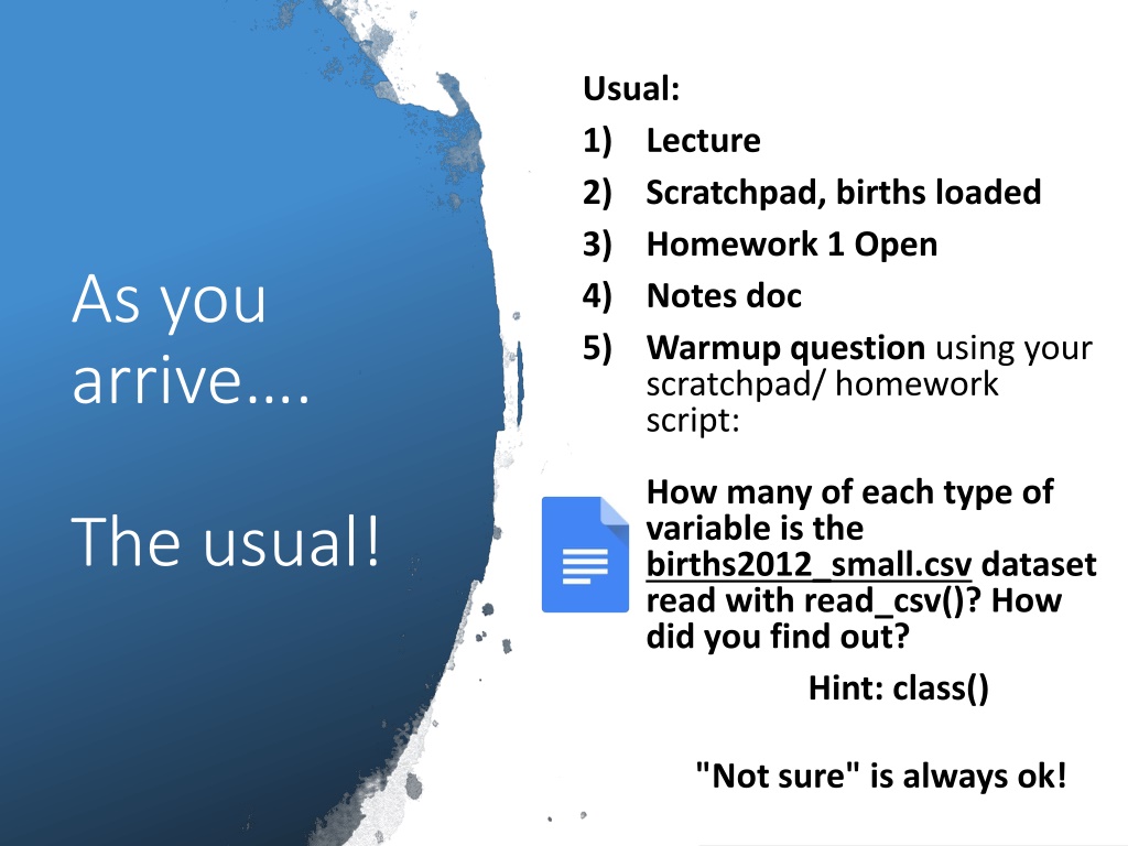
Usual: 1) Lecture 2) Scratchpad, births loaded 3) Homework 1 Open 4) Notes doc 5) Warmup question using your scratchpad/ homework script: As you arrive . How many of each type of variable is the births2012_small.csv dataset read with read_csv()? How did you find out? Hint: class() The usual! "Not sure" is always ok!
EPID 701 Spring 2020 EPID 701 Spring 2020 R for Epidemiologists R Coding III: Last of our tools: control & functions (and HW deep dive) 2020.01.23 L5 Mike learnr.web.unc.edu
1. Homework Intro! 2. Control and Functionals Today 3. Functions
Homework Homework Project Project
Motivating Question Does early prenatal care (PNC) reduce preterm birth?
Prototypical Epi Analysis Literature review Hypothesis / question generation Prepare, Explore & Recode Data (HW1*) Select / Subset Covariates (HW2) Functional Form & Crude/Basic Models (HW3) Confounding & Effect Measure Modification (HW4) Graphics & Outputs (HW5) Maps (short HW6*) Bonus stuff Nope! We re picking it. *We ll revisit some early stuff in future assignments, since some of the power of the fancier stuff you d generally apply right away! But this is the gist.
Important Epidemiology Concepts from the EPID Methods Sequence that we will be using but abbreviating hard: Exposure Outcome Risk Risk Difference/Ratio Rate Confounder Mediator Effect Measure Modifier Directed Acyclic Graphs (DAGs) for Causal Inference
DAGs Directed Acyclic Graphs (DAGs) inform our variable selection and treatment in models (based on their status as mediators, confounders, effect measure modifiers, etc. We will not elaborate in this class! Take the Epi sequence for more. DAG from EPID 716 / Christy Avery
Important Epidemiology Concepts from the EPID Methods* Sequence that we will not be using or only minimally use. Hand calculations Confidence intervals (minimal) Odds ratios DAGs .And many more! *Covered in depth in EPID 715/716 in a SAS base and the core EPID sequence.
Important Epidemiology Concepts NOT IN NOT IN the EPID Core Sequence that we will be using, because they come up a lot in public health practice, paper writing, teamwork, etc. Maps! Table & report generation Organizing a large analysis More critical analysis on disparities Etc.
Motivating Question a bit more specifically Does reduce when controlling for obvious confounders early prenatal care = PNC during or before 5th month preterm birth = less than 37 weeks Literature note: uh, only maybe sorta? It s more complex than we ll be treating it for this class. But let s mostly drop that for now! Feel free to explore the literature here. Think: PNC seems to be good. Let s figure out how good!
Relevant Variables* Exposure/Outcome Mdif: Month Prenatal Care Began Wksgest: Calculated Estimate of Gestation Covariates Mage: Maternal age Mrace: Maternal Race Methnic: Hispanic Origin of Mother Cigdur: Cigarrette Smoking During Pregnancy Cores: Residence of Mother -- County Look ahead: actually, we ll be creating some modified versions of these, but these are our base elements. And a sidenote on case / style .
Relevant Variables Selection Criteria Plur: Plurality of birth (twins, triplets, etc.) Wksgest: Calculated Estimate of Gestation DOB: Date of birth of baby Congenital Anomalies: multiple variables with congenital anomaly status (future: purrr/apply) Sex: Infant sex Visits: Total Number of Prenatal Care Visits
Control Control Quickly! Just because you can doesn't mean you should
Control To do or not to do or do repeatedly. R has traditional control structures if() {}, elseif() {}, else{}, ifelse(), for(){} Base R if_else(), case_when() Tidyverse but also benefits from vectorization!
Conditional Functions If () {} If () {} # if([BOOLEAN]){[DO STUFF]} [Boolean test] if(length(names(births)) > 10){ print ("lots of variables!") } # {} treats many statements as 1 block* # For only very short ifs (and functions) if(length(names(births)) > 10) "Bigger" else "Smaller!"
Conditional Functions Longer if else Longer if else # if([BOOLEAN]){[DO STUFF]} [Boolean test] if(file.exists("births2012_small.csv")){ print("CSV file is here!") } else if (file.exists("births_sm.rdata")){ # Optional! print("Can't find csv, but found rdata!") } else { # Optional! Note all on same line! print("Where's the file?") }
Conditional Functions dplyr dplyr:: ::if_else if_else() function () function # vectorized ifelse() # dplyr - T/F must be same type if_else( (births$ $mage[ [1: :10] ] < < 20, "Teenager", ">20") ) [Boolean test] # base - not as strict! ifelse( (births$ $mage[ [1: :10] ] < < 20, "Teenager", 20) ) # Nice for recoding! visit_tail = = tail( (births$ $visits, 20) ) if_else( (visit_tail %in% c( (88, 99) ), NA NA, visit_tail) ) births$ $visits_fixed = = if_else( (births$ $visits %in% c( (88, 99) ), NA NA, births$ $visits) ) # ^ often / next week this will be in a mutate() statement
Conditional Functions dplyr dplyr:: ::case_when case_when() () # case_when head( (births) ) births$ $smoker_mage = = case_when( (# Cascading if...else ifs...else births$ $mage < < 21 & & births$ $cigdur == == "Y" ~ ~ "Younger Smoker", births$ $mage < < 21 & & births$ $cigdur == == "N" ~ ~ "Younger Non-Smoker", births$ $mage >= >= 21 & & births$ $cigdur == == "Y" ~ ~ "Older Smoker", births$ $mage >= >= 21 & & births$ $cigdur == == "N" ~ ~ "Older Non-Smoker", TRUE TRUE ~ ~ "Something else!" # TRUE ~ to catch what's left ) ) # (Who knows what young and old is! Referencing new law @ 21) # Note the use of the Formula operator: ~ (tilde). Will see again. head( (births[ [, c( ("mage", "cigdur", "smoker_mage")]) )]) # ^ Haven't seen dplyr verbs *quite* yet!
Iteration for for - - loop by number loop by number # One approach to the warm-up we'll have more for for ( (i in in seq_along( (names( (births))){ ))){ print( (class( (pull( (births[ [,i]))) ]))) } } # ^ won't print w/o print() in for loop or function! # v Why seq_along is better than i in 1:n seq_along( (integer( (0)) )) 1: :0 Vectorization is almost always better! But how ?
Iteration for for - - loop on each string loop on each string is.numeric( (births[[ [["mage"]]) ]]) for for ( (var_name in if if( (is.numeric( (births[[ in names( (births)){ [[var_name]])){ )){ ]])){ print( (paste( (var_name, "is numeric")) print( (summary( (births[[ } } else else { { )) [[var_name]])) ]])) print( (paste( (var_name, "isn't!")) )) } } } } # See while() statement- not covering
When to (traditionally) loop Want to act quite differently on each iteration, perhaps testing as you go. Want to manage environment / memory smartly (delete duplicates as you read and combine large files, for instance) A few other cases
When NOT NOT to loop Most of the time! When you care more about the output than the "bookkeeping" When you want to do the same thing many times.
What do we need? Need some way to save complicated steps (FUNCTIONS), then vectorize more these complicated actions, AKA ITERATE ITERATE over the elements of / length of a THING THING and do STUFF STUFF. We'll get there (BRIEF intro to purrr!) after functions.
Functions that take functions as params. A powerful, compact way to iterate Functionals Functionals We'll come back to this to practice, but want you to hear the concept early. Will take repetition!
Functionals: lapply() (*apply family) in Base R lapply() (*apply family) in Base R lapply( (births, summary) ) lapply( (births, class) ) sapply( (births, class) ) Walk some list, do some thing. Would be nice to control what we're returning, have consistent syntax, be faster, and have some other conveniences purrr! https://r4ds.had.co.nz/iteration.html#the-map-functions http://adv-r.had.co.nz/Functional-programming.html
Functionals: map map functions functions - - purrr purrr in in tidyverse tidyverse # Intuition check sapply( (c( ("mike", "hillary", "your_name") ), str_to_title) ) map_chr( (c( ("mike", "hillary", "your_name") ), str_to_title) ) map_chr( (list( ("mike", "hillary", "your_name") ), str_to_title) ) # Remember a vector is a kind of (homogenous) list! # More practically: give map* a named list, get a... map( (births, class) ) # ... named char vector map_chr( (births, class) ) # ... named char vector map_lgl( (births, is.numeric) ) # ... named lgl vector map_dbl( (births[ [, map_lgl( (births, is.numeric)] )], max) ) # etc # ...see cheat sheet for more!
Functionals: map map functions functions - - purrr purrr in in tidyverse tidyverse The in functions represents a list of other parameters, often passed to another function inside. So:
Functionals: map map functions functions map2*(), map2*(), pmap pmap*() *() # More advanced: map_int( (c( (1: :5, NA), sum, na.rm=T) ) # map2_* and pmap_* versions map2_int( (1: :5, 6: :10, sum) ) pmap( (list( (n= =rep( (3,3) ), mean= =rep( (0,3) ), sd= =1: :3) ), rnorm) ) # 23 total variations...
Functions Functions
Functions: The Pipe! The Pipe! # Continuing tidyverse transition # The Pipe summary( (births) ) births %>% summary births %>% summary() () # same c( (1: :10, NA c( (1: :10, NA NA) ) %>% max NA) ) %>% max( (na.rm= =T) ) # Mike's answer to warmup! births %>% map_chr( (class) ) %>% table
Functions: Create your own reate your own # Grammar suggestions: # (1) vectors are nouns, functions are verbs. # (2) data first (pipe friendly). make_99_missing = = function function( (x){ ){ x[ [x== ==99] ] = = NA NA return( (x) ) # explicit } } make_99_missing = = function function( (x){ ){x[ [x== ==99] ] = = NA NA;x} } # ^ also valid. last operation is returned. make_99_missing( (c( (1: :4, 88, 99)) )) c( (1: :4, 88, 99) %>% ) %>% make_99_missing() ()
Functions: Create your own reate your own # hard coding '99' everywhere is bad news... make_nums_missing = = function function( (x, nums= =99){ ){ x[ [x %in% nums] ] = = NA NA;x } } make_nums_missing( (c( (1: :4, 88, 99)) )) make_nums_missing( (c( (1: :4, 88, 99) ), c( (88,99)) )) # can use names or param order c( (1: :4, 88, 99) ) %>% make_nums_missing( (c( (88,99)) )) make_nums_missing( (num = = c( (88,99) ), x= =c( (1: :4, 88, 99)) ))
Functions: Anonymous Functions Anonymous Functions # More powerful purrr - with user defined functions. numeric_births = = births[ [, births %>% map_lgl( (is.numeric)] )] numeric_births %>% map_dfc( (make_nums_missing) ) # map_dfc = get list... return Data.Frame Columns (dfc) # Functionals can use 'anonymous' functions numeric_births %>% map_dfc( (function function( (x) ) { {x[ [x == == 99]= ]=NA NA;x}) }) numeric_births %>% map_dfc(~ (~ { {.x[ [.x %in% c( (88,99)]= )]=NA NA;.x}) }) %>% tail( (20) )
Functions: Under the Hood Under the Hood #............. # How 1 function understands many classes?! summary(births); summary(births$mage) # summary() is a generic / default # that calls a class-specific version # ...simplifying a little bit, but the gist summary.data.frame(births) ?summary.data.frame # Or F1 ?summary.lm # Useful if looking for help on a function
Next Class. Starting the homework (recoding) together in earnest! (Recommend you start if you haven't already, though)
