Efficient Analysis Methods for Pipe Network Systems

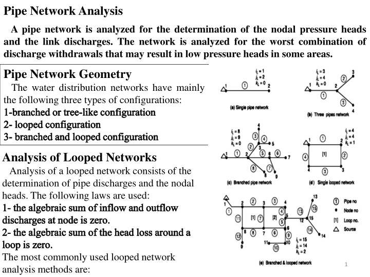
Pipe Network Analysis A pipe network is analyzed for the determination of the nodal pressure heads and the link discharges. The network is analyzed for the worst combination of discharge withdrawals that may result in low pressure heads in some areas. Pipe Network Geometry The water distribution networks have mainly the following three types of configurations: 1-branched or tree-like configuration 2- looped configuration 3- branched and looped configuration Analysis of Looped Networks Analysis of a looped network consists of the determination of pipe discharges and the nodal heads. The following laws are used: 1- the algebraic sum of inflow and outflow discharges at node is zero. 2- the algebraic sum of the head loss around a loop is zero. The most commonly used looped network analysis methods are: 1

1- Hardy Cross Method The following figure shows a relatively simple network consisting of seven pipes, two reservoirs, and one pump. The hydraulic grade lines at A and F are assumed known; these locations are termed fixed-grade nodes. Outflow demands are present at nodes C and D. Nodes C and D, along with nodes B and E are called interior nodes or junctions. Flow directions, even though not initially known, are assumed to be in the directions shown. 1-1- Generalized Network Equations Networks of piping, such as those shown in the figure can be represented by the following equations. 1. Continuity at the jth interior node: ??= ??-------(1) in which the subscript j refers to the pipes connected to a node, and Qe is the external. Use the positive sign for flow into the junction, and the negative sign for flow out of the junction. Representative piping network: (a) assumed flow directions and numbering scheme (b) designated interior loops (c) path between two fixed-grade nodes 2

2- Energy balance around an interior loop: ?? ???+ ? = ? (2) ????? ?????? ??= ?????= ????? , ??= ??= in which the subscript i pertains to the pipes that make up the loop. There will be a relation for each of the loops. The plus and minus signs in Eq.2 follow the flow in the element. If the flow is positive in the clockwise sense; otherwise, the minus sign is employed. ?: is the difference in magnitude of the two fixed-grade nodes in the path ordered in a clockwise fashion across the imaginary pipe in the pseudoloop. (HP)i is the head across a pump that could exist in the ith pipe element. If Fis the number of fixed-grade nodes, there will be (F -1) unique path equations. Let Pbe the number of pipe elements in the network, Jthe number of interior nodes, and Lthe number of interior loops. Then the following relation will hold if the network is properly defined: P = J + L + F 1 -------(3) In the figure above note that , J =4, L =2, F =2, so that P = 4 + 2 + 2 -1 = 7 3

An approximate pump head-discharge representation is given by the polynomial ??= ??+ ?? ? + ?? ??--------(4) Or, ??= ????? ? ? --------(5) It is necessary for the algebraic sign of Q to be positive in the direction of normal pump operation; otherwise, the pump curve will not be represented properly and Eq.2 will be invalid. Furthermore, it is important that the discharge Q through the pump remain within the limits of the data used to generate the curve. 1-2- Linearization of System Energy Equations Equation 2 is a general relation that can be applied to any path or closed loop in a network. If it is applied to a closed loop, ? is set equal to zero, and if no pump exists in the path or loop, (HP)i is equal to zero. Simplifying the Eq.2 to a linear form using Taylor series and neglecting second power of ?? yields ??= ?? ???+ ? = ?????? ???+ ? ? ???? ???? --------(6) ?? ?? ????? ???--------(7) Where ???? ??= ?? + ? ??? or ???? ??= 4

The Hardy Cross iterative solution is outlined in the following steps: 1. Assume an initial estimate of the flow distribution in the network that satisfies continuity, Eq.1. 2. For each loop or path, evaluate ?with Eq.6 ??= ?? ??? ? = ?????? ???+ ? ? ???? ???? --------(6) ?? ?? 3. Update the flows in each pipe in all loops and paths, such that: ?? ???= ?? ???+ ?? --------(8) The term ?? is used, since a given pipe may belong to more than one loop; hence the correction will be the sum of corrections from all loops to which the pipe is common. 4. Repeat steps 2 and 3 until a desired accuracy is attained. One possible criterion to use is ?? ??? ?? ? in which ? is (0.001 < ? < 0.005) 5

Example 1: The pipe network of two loops as shown in Fig. 3.11 has to be analyzed by the Hardy Cross method for pipe flows for given pipe lengths L and pipe diameters D. The nodal inflow at node 1 and nodal outflow at node 3 are shown in the figure. Assume a constant friction factor f = 0.02. Solution There are four junctions (J =4), five pipes (P =5), and (F=0). Hence the number of closed loops is : L = P - J - F + 1 L =5 -4 -0 +1 =2. The two loops and assumed flow directions are as shown. Equation 6 is applied to each loop as follows: To apply continuity equation for initial pipe discharges, the discharges in pipes 1 and 5 equal to 0.1 m3/s are assumed. Th e obtained discharges are Q1 = 0.1 m3/s (flow from node 1 to node 2) Q2 = 0.1 m3/s (flow from node 2 to node 3) Q3 = 0.4 m3/s (flow from node 4 to node 3) Q4 = 0.4 m3/s (flow from node 1 to node 4) Q5 = 0.1 m3/s (flow from node 1 to node 3) ??? ?????? ???? ? ??= ?????? ???+ ? ? ???? ???? ??= ??????+??????+?????? ?????+?????+????? ??= ??????+??????+?????? ?????+???? +????? ?? 6 ?? ???= ?? ??? ?? ??

Curve =1 Curve = 2 Type a0 250 Power . Kw 20.000 1 Example 1 a1 -0.4 Gama 9.800 a2 -0.1 Iteration 1 Gi =2K Q - dHp/dQ Pump Position Common Pipe Wi = K Q Q + Hp Qi = Qo+ Qi Pipoe no. L f D Ri Ki Qo Hp Loop I Delta H 0 Pipe 3 300 0.02 0.1 0 49576.114 -0.4 0.00 -7932.1783 39660.8915 -0.2540 Pipe 4 200 0.02 0.15 0 4352.3612 -0.4 0.00 -696.3778 3481.8890 -0.2540 Pipe 5 2 360 0.02 0.1 0 59491.337 0.1 0.00 594.9134 11898.2675 0.2359 Sum -8033.6427 55041.048 Q1 Q2 0.145957 0.01005 0.14596 Q1 Gi =2K Q - dHp/dQ Pump Position Common Pipe Wi = K Q Q + Hp Qi = Qo+ Qi Pipoe no. L f D Ri Ki Qo Hp Loop II Delta H 0 Pipe 1 0 300 0.02 0.15 0 6528.5418 0.1 0.00 65.2854 1305.7084 0.1100 Pipe 2 0 200 0.02 0.1 0 33050.743 0.1 0.00 330.5074 6610.1486 0.1100 Pipe 5 0 1 360 0.02 0.1 0 59491.337 -0.1 0.00 -594.9134 11898.2675 -0.2359 Sum -199.1205 19814.124 Q1 Q2 0.14596 0.01005 0.01005 Q2 7

Example 1 Iteration 2 Iteration 3 Gi =2K Q - dHp/dQ Wi = K Q Q + Hp Gi =2K Q - dHp/dQ Qi = Qo+ Qi Wi = K Q Q + Hp Qi = Qo+ Qi Qo Hp Qo Hp Loop I Loop I 0 0 Pipe 3 -0.2540 0.00 -3199.5281 25188.9000 -0.2510 Pipe 3 -0.2510 0.00 -3122.9859 24885.7794 -0.2114 Pipe 4 -0.2540 0.00 -280.8914 2211.3712 -0.2510 Pipe 4 -0.2510 0.00 -274.1716 2184.7598 -0.2114 Pipe 5 0.2359 0.00 3310.8432 28068.9501 0.1620 Pipe 5 0.1620 0.00 1560.9200 19272.9054 0.1964 Sum -169.5762 Sum -1836.2374 46343.4445 55469.22124 0.00306 0.039622 Q1 Q1 Q1 Q2 Q1 Q2 0.003057 0.076984 0.039622 0.005176 Gi =2K Q - dHp/dQ Wi = K Q Q + Hp Gi =2K Q - dHp/dQ Qi = Qo+ Qi Wi = K Q Q + Hp Qi = Qo+ Qi Qo Hp Qo Hp Loop II Loop II 0 0 Pipe 1 0.1100 0.00 79.0664 1436.9245 0.1870 Pipe 1 0.1870 0.00 228.3788 2442.1140 0.1922 Pipe 2 0.1100 0.00 400.2734 7274.4304 0.1870 Pipe 2 0.1870 0.00 1156.1674 12363.2023 0.1922 Pipe 5 -0.2359 0.00 -3310.8432 28068.9501 -0.1620 Pipe 5 -0.1620 0.00 -1560.9200 19272.9054 -0.1964 Sum -2831.5034 Sum -176.3738 36780.30501 34078.2217 0.07698 0.005176 Q2 Q2 8

Example 1 Iteration 4 Iteration 5 Gi =2K Q - dHp/dQ Gi =2K Q - dHp/dQ Wi = K Q Q + Hp Qi = Qo+ Qi Wi = K Q Q + Hp Qi = Qo+ Qi Qo Hp Qo Hp Loop I Loop I 0 0 Pipe 3 -0.2114 0.00 -2214.7833 20957.1324 -0.2089 Pipe 3 -0.2089 0.00 -2163.4183 20712.6890 -0.1978 Pipe 4 -0.2114 0.00 -194.4391 1839.8580 -0.2089 Pipe 4 -0.2089 0.00 -189.9297 1818.3979 -0.1978 Pipe 5 0.1964 0.00 2295.4017 23371.4799 0.1773 Pipe 5 0.1773 0.00 1870.1414 21095.7067 0.1868 Sum -113.8207 Sum -483.2066 46168.4703 43626.794 0.0024653 0.0110759 Q1 Q1 Q1 Q2 Q1 Q2 0.002465 0.0215923 0.011076 0.0016026 Gi =2K Q - dHp/dQ Gi =2K Q - dHp/dQ Wi = K Q Q + Hp Qi = Qo+ Qi Wi = K Q Q + Hp Qi = Qo+ Qi Qo Hp Qo Hp Loop II Loop II 0 0 Pipe 1 0.1922 0.00 241.1929 2509.6917 0.2138 Pipe 1 0.2138 0.00 298.4266 2791.6237 0.2154 Pipe 2 0.1922 0.00 1221.0392 12705.3144 0.2138 Pipe 2 0.2138 0.00 1510.7848 14132.5951 0.2154 Pipe 5 -0.1964 0.00 -2295.4017 23371.4799 -0.1773 Pipe 5 -0.1773 0.00 -1870.1414 21095.7067 -0.1868 Sum -833.1696 Sum -60.9299 38586.4861 38019.926 0.0215923 0.0016026 Q2 Q2 9

Example 1 Iteration 6 Gi =2K Q - dHp/dQ Wi = K Q Q + Hp Qi = Qo+ Qi Qo Hp Loop I 0 Pipe 3 -0.1978 0.00 -1940.0881 19614.4874 -0.1970 Pipe 4 -0.1978 0.00 -170.3232 1721.9852 -0.1970 Pipe 5 0.1868 0.00 2075.3271 22222.8696 0.1815 Sum -35.0842 43559.342 0.0008054 Q1 Q1 Q2 0.000805 0.0060827 Gi =2K Q - dHp/dQ Wi = K Q Q + Hp Qi = Qo+ Qi Qo Hp Loop II 0 Pipe 1 0.2154 0.00 302.9172 2812.5487 0.2215 Pipe 2 0.2154 0.00 1533.5183 14238.5279 0.2215 Pipe 5 -0.1868 0.00 -2075.3271 22222.8696 -0.1815 Sum -238.8916 39273.946 0.0060827 Q2 10