Digital Signal Processing I 4th Class 2020-2021 by Dr. Abbas Hussien & Dr. Ammar Ghalib
This content delves into Digital Signal Processing concepts taught in the 4th class of 2020-2021 by Dr. Abbas Hussien and Dr. Ammar Ghalib. It covers topics like Table Lookup Method, Linear Convolution, Circular Convolution, practical examples, and Deconvolution techniques such as Polynomial Approach. The material includes graphical representations, equations, and explanations to aid in understanding the subject.

Download Presentation

Please find below an Image/Link to download the presentation.
The content on the website is provided AS IS for your information and personal use only. It may not be sold, licensed, or shared on other websites without obtaining consent from the author.If you encounter any issues during the download, it is possible that the publisher has removed the file from their server.
You are allowed to download the files provided on this website for personal or commercial use, subject to the condition that they are used lawfully. All files are the property of their respective owners.
The content on the website is provided AS IS for your information and personal use only. It may not be sold, licensed, or shared on other websites without obtaining consent from the author.
E N D
Presentation Transcript
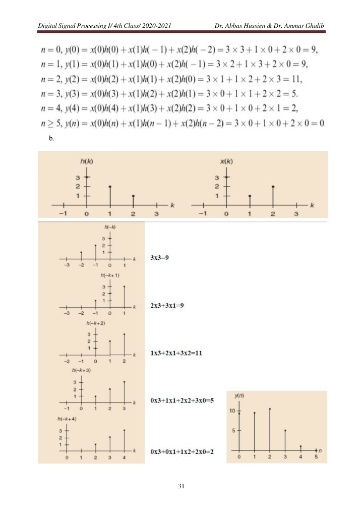
Digital Signal Processing I/ 4th Class/ 2020-2021 Dr. Abbas Hussien & Dr. Ammar Ghalib b. 31
Digital Signal Processing I/ 4th Class/ 2020-2021 Dr. Abbas Hussien & Dr. Ammar Ghalib Table LookupMethod: Matrix by Vector Method: Linear Convolution and Circular Convolution: Linear convolution: Circular convolution: Note: If both x (n) and x (n) are of finite length N and N and defined on [0 N 1] and [0 N 1] 1 2 respectively, the value of N needed so that circular and linear convolution are the same on [0 N- 1 2 1 2 1] is: N N + N 1 1 2 32
Digital Signal Processing I/ 4th Class/ 2020-2021 Dr. Abbas Hussien & Dr. AmmarGhalib Example: If x(n) = [1 2 3 2], and h(n) = [1 1 2]. Find y(n) such that linear and circular convolution are the same. sol. N = 4 + 3 1 = 6 Then x(n) = [ 1 2 3 2 0 0 ] and h(n) = [ 1 1 2 0 0 0] x(n) is arranged in clockwise direction ,while h(n) is arranged in the opposite clockwise direction (bold numbers). Each time, only h(n) will be shifted with the clockwise direction to find y(n). Note: the reference point is * and, the arrows represent multiplication process. Finally, addition process is performed. 1 1 0 2 1 0 x(n) h(n) 0 2 0 3 0 2 1 1 1 1 1 2 2 2 2 0 0 0 0 1 1 1 2 0 h(n) h(n) h(n) 1 0 0 2 0 0 3 3 0 0 3 0 0 0 0 2 2 2 1 0 1 0 1 0 2 2 2 0 0 0 2 0 0 1 0 0 h(n) h(n) 1 2 0 0 1 1 3 3 0 0 3 0 1 1 2 2 2 2 Example: Use graphical method to find circular convolution of x (n)=[1 2 2] and x (n)=[0 1 2 3]. 1 2 sol. Applying the equation of circular convolution 33
Digital Signal Processing I/ 4th Class/ 2020-2021 Dr. Abbas Hussien & Dr. Ammar Ghalib y(0) = x (0) x (0) + x (1) x (3) + x (2) x (2) + x (3) x (1) = 1(0) + 2(3) + 2(2) + 0(1) = 10 1 2 1 2 1 2 1 2 and so on Deconvolution: The digital Deconvolution can be performed by Iterative Approach, Polynomial Approach, and Graphical Method. In the following subsection, the polynomial approach will be explained. PolynomialApproach: A long division process is applied between two polynomials. For causal system, the remainder is always zero. If y(n) = [12 10 14 6] and h(n) = [4 2] 2 3 Then y = 12 + 10 x + 14 x + 6 x , and h = 4 + 2 x. Applying long division, we obtain 2 i/p = 3 + x + 3 x . Then x(n) = [3 1 3] 34