Overview of Digital Signal Processing (DSP) Systems and Implementations
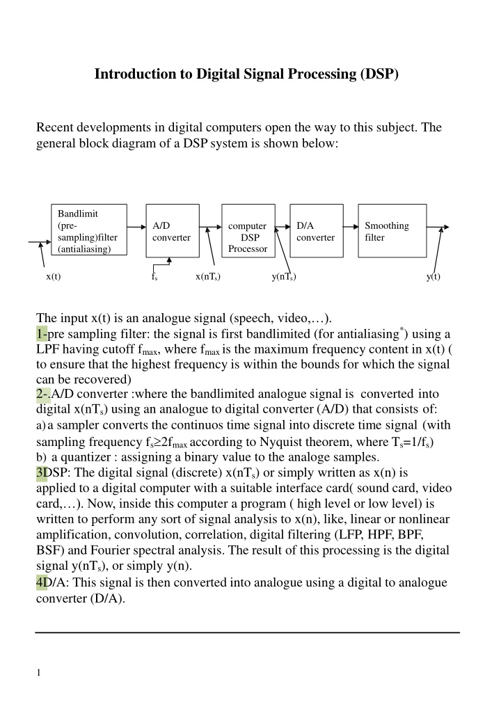
Recent advancements in digital computers have paved the way for Digital Signal Processing (DSP). The DSP system involves bandlimiting, A/D conversion, DSP processing, D/A conversion, and smoothing filtering. This system enables the conversion of analog signals to digital, processing using digital computers, and reconversion back to analog. DSP systems can be linear or nonlinear and causal or non-causal, allowing for a wide range of signal processing applications. Software implementation provides flexibility in design, and modern technology enables complex systems to be implemented on a single silicon chip.

Download Presentation

Please find below an Image/Link to download the presentation.
The content on the website is provided AS IS for your information and personal use only. It may not be sold, licensed, or shared on other websites without obtaining consent from the author.If you encounter any issues during the download, it is possible that the publisher has removed the file from their server.
You are allowed to download the files provided on this website for personal or commercial use, subject to the condition that they are used lawfully. All files are the property of their respective owners.
The content on the website is provided AS IS for your information and personal use only. It may not be sold, licensed, or shared on other websites without obtaining consent from the author.
E N D
Presentation Transcript
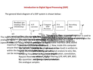
Introduction to Digital Signal Processing (DSP) Recent developments in digital computers open the way to this subject. The general block diagram of a DSP system is shown below: Bandlimit (pre- sampling)filter (antialiasing) A/D converter D/A converter Smoothing filter computer DSP Processor x(t) fs x(nTs) y(nTs) y(t) The input x(t) is an analogue signal (speech, video, ). 1-pre sampling filter: the signal is first bandlimited (for antialiasing*) using a LPF having cutoff fmax, where fmax is the maximum frequency content in x(t) ( to ensure that the highest frequency is within the bounds for which the signal can be recovered) 2-.A/D converter :where the bandlimited analogue signal is converted into digital x(nTs) using an analogue to digital converter (A/D) that consists of: a)a sampler converts the continuos time signal into discrete time signal (with sampling frequency fs 2fmax according to Nyquist theorem, where Ts=1/fs) b) a quantizer : assigning a binary value to the analoge samples. 3DSP: The digital signal (discrete) x(nTs) or simply written as x(n) is applied to a digital computer with a suitable interface card( sound card, video card, ). Now, inside this computer a program ( high level or low level) is written to perform any sort of signal analysis to x(n), like, linear or nonlinear amplification, convolution, correlation, digital filtering (LFP, HPF, BPF, BSF) and Fourier spectral analysis. The result of this processing is the digital signal y(nTs), or simply y(n). 4D/A: This signal is then converted into analogue using a digital to analogue converter (D/A). 1
5- smoothing filter: a smoothing filter is used to remove the staircase shape of y(n) to give the continuous output signal y(t). The software implementation of the signal analysis on x(n) gives high flexibility in design and processing. With the recent advances in digital technologies it is possible to implement very complicated systems on a single general purpose silicon chip. Classification of DSPsystems: According to the relation between the output y(n) and the input x(n), any DSP system can be classified according to the following: 1-Linearity: A DSP system is called linear if the superposition theorem applies. Superposition means that sum of the input= sum of the output. Figure below illustrated that the system output due to the weighted sum inputs x1(n)+ x2(n) is equal to the same weighted sum of the individual outputs obtained from their corresponding inputs, that is,y(n)= y1(n)+ y2(n). System x1(n) y1(n) System y2(n) x2(n) x1(n)+ x2(n) y1(n)+ y2(n) System Digital linear system Example1 if y(n)= 2x(n) which is a simple DSP system representing an amplifier with gain=2. This DSP system is linear since superposition applies here, if x(n)=x1(n)+x2(n), then: y(n)=2[x1(n)+x2(n)]=2 x1(n)+2x2(n)=y1(n)+y2(n), where y1(n) and y2(n) are the outputs due to x1(n) and x2(n) if they are applied one at a time. Example2 y(n)=3e0.2x(n) which is a DSP system representing an exponential amplifier, now if x(n)=x1(n)+x2(n), then: y(n)=3e0.2[x (n)+x (n)]= 3e0.2x1(n) e0.2x2(n) y (n)+y (n), this system is nonlinear. Note : examples for the nonlinear systems are: y(n)= ln(x(n)), y(n)=sin(x(n)), y(n)=1/ x(n) , y(n)= (x(n))2 1 2 1 2 2
2 Causality: A DSP system is said to be causal if the present value of y [ i.e. y(n)] is not a function of some future values of x [i.e. x(n+i), i, +ve integer] or some future values of y [i.e. y(n+i), i, +ve integer]. The causal DSP system that is physically realizable is that system where y(n) is a function of present value of x(n) or some previous values of x [i.e x(n-i) ,i, +ve integer] or some previous values of y [i.e. y(n-i), i +ve integer]. In other words, a causal system is one where response does not begin before the input signal is applied. Example1: if y(n)=3x(n)-2x(n-1)+y(n-3)+ex(n) which is not linear due to the exponential term but it is causal since y(n) is not a function of some future terms of x or y. Example2: y(n)=x(n+1)-x(n)+3y(n+3) is not causal and is not physically realizable since y(n) depends on some future values of x and y, [these are x(n+1)) and y(n+3)]. Note : examples of the noncausal systems are: y(n)=x(n+1), y(n)=x(n2) , y(n)=x(-n), y(n)=x n . 3 Stability: A DSP system is said to be stable if the O/P is bounded for bounded I/P (bounded input gives bounded output BIBO). Ex1: if y(n)=2x(n)-0.5x(n-1), and |x(n)|<G where G is finite, then |y(n)|<2G- 0.5G or |y(n)|<1.5G. hence if x(n) is bounded by G then y(n) is also bounded i.e. the system is stable. Ex2: y(n)=ex(n-1) which is a nonlinear causal system, then if |x(n)|<G, then |y(n)|<eGand if G is finite, then y(n) is bounded, i.e., the system is stable. Stability of linear DSP system can be studied usually in terms of transfer function in z-domain, H(z)=Y(z)/X(z) Where the z-transforms of x(n) and y(n) are: X (z) = x(n)z n n= Y(z) = y(n)z n n= If H(z) has pole(s) outside the unit circle (|z|=1), then the system is unstable, otherwise, it is a stable system. Poles on the unit circle gives critically stable. 3
Im z unstable unstable Rez Stable 1 unstable unstable Ex: If y(n)=2x(n-1) 3x(n). Check if this system is stable or not. Solution: Taking Z-transform of both sides, get: Y(z)=2z-1X(z)-3X(z) (using shift property of z-transform) Or Y(z)/X(z)=H(z)=2z-1-3 or: H(z)=(2-3z)/z which has a single pole at z=0(inside the unit circle), hence this system is stable. Ex: check the stability of the system: y(n)=x(n)+2y(n-1), Solution:As before, taking the z-transform of both sides and using the shift property, then : Y(z)=X(z)+2z-1Y(z), or Y(z)[1-2z-1]=X(z), then: H(z)=Y(z)/X(z)=1/(1-2z-1)=z/(z-2) which has a pole at z=2(outside the unit circle, hence this system is unstable. 4-Time Variant-Time Invariant DSP system: A time variant system is that system with time varying characteristics that depends on the time index n. For example, y(n)=n x(n) is a time variant system. In fact, this system is an amplifier having variable gain with time. Take another example say y(n)=2e-x(n-1)which is a nonlinear, causal, stable system. This system is time invariant since its characteristics do not change with time index n. Ex: Classify the following DSP system for linearity, causality, stability and time invariant: y(n)=2ex(n)-n x(n-2) + y(n-2). Solution: This system is: -nonlinear due to the exponential term. -casual since y(n) does not depend on some future terms of x or y. 4
-unstable due to the term n x(n-2) which is unbounded with time index n even if x is bounded. -time variant due to the n x(n-2) term. Homeworks: classify the following DSP systems for linearity, causality, time-invariance and stability: a) y[n] = 3 x(n) 4 x(n-1) b) y[n] = 2 y(n-1) + x(n+2) c) y[n] = n x(n) d) y[n] = cos (x(n)) e) y[n] = log10(x(n)) f) y[n] = x[n]4 Input/output relations of the linear systems: a) Analogue (continuous)systems(review): If h(t) is the impulse response, where t is the time index. H(w) is the transfer function which is the Fourier transform of h(t). y(t)=x(t) h(t) Where is the convolution: t y(t) = x( ) h(t ) d = h( ) x(t ) d 0 Also: Y(w)=X(w) H(w) and: |Y(w)|2 = |X(w)|2 |H(w)|2or y(t) x(t) h(t) H(w) Y(w) X(w) t 0 Gy(w)=Gx(w) |H(w)|2 where Gx(w) and Gy(w) are spectral densities of x and y respectively. Also output power y 2 (t) = | H (w) |2 G (w) dw x 5
b) Discrete (digital) systems: Here h(n) is the impulse response of the System,where n is the time index, and H(z) is its transfer function: H(z)=Y(z)/X(z) And: y(n)=x(n) h(n) or: y(n) = x(n) h(n k) = h(k) x(n k) k which is called the discrete convolution. DSP systems are classified according to their impulse responses h(n) into: x(n) y(n) h(n) X(z) Y(z) H(z) k a) FIR (Finite Impulse Response): where h(n) has finite number of elements such as: h(n)={1,2,4,3,0,1} where the cursor indicates the position where n=0. h(n) 4 3 2 1 1 n b)IIR(Infinite Impulse Response): where h(n) has infinite number of elements such as: h(n)=( )n u(n) where u(n) is the unit step function: u(n)= 1 for n=0,1,2,3, 0 elsewhere u(n) 1 n h(n) 1 0.5 0.25 0.125 n 6
Discrete convolution Methods: 1- Graphical method: This includes the basic convolution steps :- reversing in time using k as time index, -shifting by n samples, -multiplication of the corresponding samples, -addition . x(k) 3 2 1 Ex: h(n)={1,-1,2}, x(n)={2,1,-1,3}. k -1 y(n) = x(k)h(n k) k y(0) = x(k)h(0 k)=2+(-1)(-1)+(1)(3)=6 k h(-k) 2 1 y(1)= x(k)h(1 k)=2(-1)+(-1)(3)=-5 k k y( 1) = x(k)h( 1 k)=(2)(2)+(-1)(1)+(1)(-1)=2 k And so on, shifting of h(n) (left and right) until the overlapping between x(k) and h(n-k) disappears giving 0's at the output y(n). -1 h(1-k) 2 1 k -1 h(-1-k) 2 1 k -1 7
2-Tabular Method: This is a very simple method used for FIR systems with finite number of samples x(n). A rectangular table with N1 rows (no of elements in h(n)) and N2 columns(no of elements in x(n)), or visa versa, is arranged. Then, the cross multiplications are carried out. The sum of multiplications diagonally will give the values of y(n). Ex: Repeat previous example using tabular method. h(n)={1,-1,2}, x(n)={2,1,-1,3}. 2 2 -2 4 1 1 -1 2 -1 -1 1 -2 3 3 1 -1 2 -3 6 Then y(n)={2,-1,2,6,-5,6} Note that N=N1+N2-1=no of elements in y(n) =3+4-1=6 If O1 and O2 are positions of the cursors in h(n) and x(n)(from the left), then O=O1+O2-1=position of the cursor(position of y(0)) in y(n) =2+3-1=4 3-Add-overlap method: This is a modified method from the tabular method, when either h(n) or x(n) has large no of elements, then this can be divided into subsegments of smaller length. This helps to save memory. Ex: Find the discrete convolution between: h(n)={1,-1,2} and x(n)={1,2,-1, 3,4,-1,0,3} solution: Here x(n) is divided into segments of length 3 (say), with the last segment will be of length 2 (no problem). Hence previous tabular method is repeated 3 times: 8
1 1 2 -1 -1 -1 -2 1 2 2 4 -2 1 2 -1 y1(n)={1,1,-1,5,-2} 1 3 4 -1 -1 -3 -4 1 2 6 8 -2 3 4 y2(n)={3,1,1,9,-2} -1 1 0 3 -1 0 -3 2 0 6 0 3 y3(n)={0,3,-3,6} Then, add y1, y2, and y3 , with y2 shifted to the left by 3 elements(length of each segment) and y3 shifted to the left by 6 elements ,i.e.: 1 1 -1 5 -2 y1 y2 y3 3 1 1 9 -2 3 0 -3 6 sum y(n)={ 1, 1, -1,8 , -1, 1, 9, 1 , -3, 6} with the cursor for y(n) at O=2+4-1=5 4- Matrix method: Here, [Y]=[A][h], where [Y]T=[y(n)]=output, [h]T=[h(n)] and the matrix [A] has N=N1+N2-1 rows and N2 columns(no of elements of h(n)). The 1st rowin [A] is the 1st element in x(n)(from the left) and the remaining elements are 0's. The 2nd row in [A] is the 2nd element in x(n), then the 1st element in x(n) and the remaining elements are 0's. and so on until the last element in x(n) is entered at the N1th row( N1 is the no of elements in x(n)). After that 0's are applied in stead of the elements of x(n) until the last row at N=N1+N2-1. 9
Ex: h(n)={1,-1,2}, x(n)={2,1,-1,3} Solution: 2 2 1 1 0 0 2 2 1 1 0 0 0 2 1 2 0 1 1 2 1 1 2 1 1 = [h] = 1 1 [ A] = 3 1 2 then:[Y]= 3 6 1 3 1 3 0 0 0 2 5 1 0 6 0 0 3 3 Or y(n)={2,-1,2,6,-5,6} where O=2+2-1=3 5-The Z-transform method: This is a general method used when either or both of h(n) and x(n) has infinite elements.(Note if both h(n) and x(n) has finite no of elements then use the tabular method since it is very simple). The procedure here is to take the z-transform of x(n) and h(n), then multiply to find Y(z) from which y(n) is found using inverse z-transform. Ex: h(n)={1,-1,2}, x(n)=( )nu(n). Solution: Note, since x(n) has infinite no of elements, then, we must use z- transform method. Now, taking the z-transforms of h(n) and x(n), then: H (z) = h(n) z n =1. z1+(-1).z0+2.z-1=z-1+2z-1. n= 1 X (z) = x(n) z n= (0.5)nz n= (0.5z 1)n n= n=0 X (z) = 1= z (recall that in general Z[anu(n)]=z/(z-a) ) Then Y(z)=H(z).X(z)=[z-1+2z-1][z/(z-0.5)] 2 + =z 0.5 z 0.5 z 0.5 And y(n)=(0.5)n+1u(n+1) (0.5)n u(n) +2 (0.5)n-1u(n-1) Note: recall the shift property Z[x(n-a) u(n-a)]=X(z) z-a. 1 or: n=0 z 0.5 1 0.5z 1 z . z z 11
Ex: Find 1- (n-a)(n-b) 2- (n-a) u(n-b) z-transform and for real constants a & b. ( (n) is the delta dirac function). Solution: 1- Z[ (n-a)]=z-a and Z[ (n-b)]=z-b, then: Z-1[z-a z-b]= Z-1[z-(a+b)]= (n-{a+b}) Hence: (n-a) (n-b) = (n-{a+b}). 3- u(n-a) u(n-b) using the 2- Z[ (n-a)]=z-a and Z[u(n-b)]=z-b z/(z-1), then: Z-1[z-a z-b z/(z-1)]= Z-1[z-(a+b) z/(z-1)]= u(n-{a+b}) Hence: (n-a) u(n-b) = u(n-{a+b}). 3- Z[u(n-a)]=z-a z/(z-1), Z[u(n-b)]=z-bz/(z-1), Z-1[z-a z/(z-1) z-b z/(z-b)]= Z-1[z-(a+b-1)z/(z-1)2] = (n-{a+b-1})u(n-{a+b-1}) which is a ramp function. (Note: recall that Z[n u(n)]=z/(z-1)2 Hence: u(n-a) u(n-b) = (n-{a+b-1})u(n-{a+b-1}) ). Homeworks: 1- find Z [sin 0n] and Z [cos 0n]. 2- find an u(n) u(n). 6-Frequency Response of the DSP system: If x(n) = Ae j o n (sampled sinusoid),then: y(n) = h(k)x(n k) or: k y(n) = h(k) A ej o(n k)= Aej o n h(k) e j o k k h(k) e = H ( ) h(n) x(n) y(n) k j ok o which is the frequency response of h(n) at = o If k of the input sinusoid. Or in general, H ( ) = h(k) e j k= |H( )| ( ) with magnitude and phase values. k So, the output y(n) can be easily obtained as: y(n) = x(n) |H( )| ( ) 11
Ex: For the DSP system shown, if x(t)=10cos(300t), find x(n) and y(n). h(n)=(0.5)nu(n) A/D D/A y(t) x(t) fs=1KHz Solution: fs=1000 Hz, then Ts=1/fs=0.001, t=nTs, then: x(nTs) = x(n) =10 cos(300 (0.001n))=10 cos(0.3 n). hence, the input is a discrete sampled sinusoid with o=0.3 rad . To find y(n), we use the frequency response method since its much easier than the z-transform method. Then: y(n) = x(n) |H( )| ( ) H ( ) = h(k) e j k= (0.5)k e j k= (0.5e j )k k k=0 1 Then: H (w) =1 0.5e jw 1 Simplify: H ( ) =1 0.5cos + 0.5jsin 1 1 cos +0.25cos2 +0.25sin2 ( ) = tan 1 0.5sin Where k=0 1 (recall geometric series r = k ) 1 r k=0 1 | H( ) |= = 1.25 cos 1 0.5cos x(n)=10 cos(0.3 n), then = o=0.3 rad. For 1 | H(0.3 )|= = 1.228and 1.25 cos(0.3 ) (0.3 ) = tan 1 0.5sin(0.3 ) rad 6 1 0.5cos(0.3 ) Then y(n) = 10 * 1.228 cos(0.3 n) - /6 =12.28cos{0.3 n-( /6)} 12
Discrete Deconvolution: To find h(n) if both x(n) and y(n) are given. x(n) h(n) y(n) Here, we usually use the z-transform method since it is valid for both the FIR and IIR DSP systems. h(n)= Z-1[H(z)]= Z-1[Y(z)/X(z)] Ex: find h(n) if x(n)={ 1,-1,3} and y(n)={2,3,-1,17,-6} Solution: X(z)=1-z-1+3z-2 and Y(z)= 2+ 3z-1 -z-2 +17z-3- 6z-4. Then, using the long division: 2+5z-1 -2z-2 2+ 3 z-1 z-2 +17z-3-6z-4 2 - 2z-1 +6z-2 5z-1 7z-2 +17z-3-6z-4 5z-1 - 5z-2+15z-3 -2z-2 +2z-3-6z-4 -2z-2 +2z-3 -6z-4 0 1-z-1 + 3z-2 0 0 Hence: H(z)= 2+5z-1 -2 z-2 or then, the system is FIR. h(n)={2,5,-2} and since there is no remainder, Ex: Find h(n) if x(n)=u(n) and y(n)=2u(n)-(0.5)nu(n). Solution: X(z)=z/(z-1) and Y(z)= [2z/(z-1)] [z/(z-0.5)] 2z z Then H (z) =z 1 z 0.5= 2 z 1 =2z 1 z +1= z z z 0.5 z 0.5 z 0.5 z 1 Hence h(n)=(0.5)nu(n). 13
DSP system Implementations a) FIR systems: Here h(n) has finite no of elements: h(n)={h(0), h(1), h(2), ..,h(m)} with (m+1) elements. H(z) = h(0) + h(1) z-1 + h(2) z-2 + .+ h(m) z-m and if : H(z)=Y(z)/X(z), then: y(n) = h(0) x(0) + h(1) x(n-1) + h(2) x(n-2) + .+ h(m) x(n-m) i.e., y(n) is obtained from x(n) by the weighted sum (weighted by h(n)) of the delayed samples of x(n). These delayed samples of x(n) are obtained using a tapped delay line with m-taps and with Ts time delay pertap. z-1 z-1 z-1 z-1 z-1 z-1 .. z-1 Ts .. x(n) h(0) h(m) h(1) y(n) Note that the FIR system is always stable, (no poles outside the unit circle), or we say that the FIR system is an open loop without a feedback and that is why it is called nonrecursive. b)-IIR system: For IIR system having m-zeros and r-poles, then: Y(z) a + a z 1 + a z 2 + .......... . + az m = H (z)= 1 2 o m 1+b z 1+ b z 2+........ + b z r 1 2 X(z) r Where, we can always set the 1st term at the denominator to unity by dividing with a suitable constant (say bo). From which: y(n)=aox(n)+a1x(n-1)+a2x(n-2)+ .+amx(n-m)- b1y(n-1)- b2y(n-2)- .- bry(n-r) Note that y(n) depends on present and previous values of x and on previous values of y. Hence: 1 IIR system contains a feedback from the output to the input. 2 possibility of instability if some poles of H(z) lies outside the unit circle. 14
3- To implement the IIR system, then 2 tapped delay lines are required, one with m-taps for the x input and the other with r-taps for the feedback from the y output. y(n) x(n) z-1 b1 z-1 z-1 z-1 z-1 z-1 z-1 z-1 z-1 z-1 z-1 z-1 z-1 br Ex: Implement the DSPsystem: 4 2z 2 H (z)= 2+3z 1 z 2+ z 3 Solution: This is an IIR system. Dividing by 2 to set the 1st term at the denominator to unity, then: H(z) = This needs a tapped delay line with 2 taps for x 1+1.5z 1 0.5z 2+ 0.5z 3 and a tapped delay line with 3 taps for y. 2 z 2 x(n) y(n) z-1 z-1 z-1 z-1 z-1 15
Spectral Analysis of Discrete Signals: a-periodic discrete signals: If x(n) is a periodic signal having a period of N samples, i.e. x(n) is repeated every N samples, then the frequency content of x(n) (spectral analysis) is obtained using discrete Fourier series (DFS), where: N 1 n=0 x(n)e N where n is the time index and k is the frequency index, i.e.: X(0)=dc component. X(1)=1st harmoniccomponent. X(2)=2nd harmonic component and so on up to the N-1 harmonic component X(N-1). x(n) = X(k)e j2 n k 1 X(k) = N N- 1 k 0 j 2 n k N 1 N N- 1 n 0 The inverse DFS is given by: k=0 Ex: Find the DFS of the signals x(n) shown: Solution: x(n) n Note that x(n) is periodic with period N=4 samples and is defined for full period by: x(n)={2,-1,3,-3}. Then: 1 =x(0) + x(1) + x(2) + x(3) 4n=0 j 2 n(0) 2 1+ 3 3 3 1 4 X(0) = x(n)e = = 4 =dc value 4 4 16
j3 j j 2 n(1) 1 4n=0 1 3 X(1) = x(n)e j = [x(0) +x(1)e + x(2)e + x(3)e 2] 4 2 4 X(1)=0.25[2-1(-j)+3(-1)-3(j)] = 0.25(-1-2j) = -0.25-0.5j Similarly, we find X(2)=9/4 and X(3)=-0.25+0.5j Note that X(3)=X*(1) (* conjugate) It should be noted, however, that the discrete behavior of DFS directly gives the discrete line spectrum of Fourier series analysis with k index being the harmonic number. Also this frequency index is for N- 1 k 0 , i.e. for N- sampled periodic signal, the harmonic analysis is done up to (N-1). b- aperiodic or random discrete signals: If x(n) is aperiodic or random, such as pulses, speech, video, .. when sampled at fs then spectral analysis is done for finite segment (length) of such signals, i.e. N samples are taken from such a signal ( this corresponds to NTs time interval from x(t)). Here, we use the discrete Fourier transform (DFT). x(t) x(N-1) x(0) N samples If x(n)={x(0), x(1),x(2), .x(N-1)} is the sampled signal from x(t), then the DFT of x(n) is given by: j2 n k N 1 x(n)e n=0 1 N X(k) = N N- 1 k 0 j 2 n k N 1 And the inverse DFT (IDFT) is:x(n) = X(k)e N k=0 Theoretically, x(t) has continuous spectrum, but due to sampling at fs, then this will give a discrete approximation to this continuous spectrum by X(k). 17
The relation between frequency in Hz and the frequency index k is given by the frequency resolution between successive values of k, this is given by: frequncyresolution=fs N Such that the discrete behavior of |X(k)| approaches the continuous spectrum as N . |X(k)| k N/2 N N-1 fs/2 fs fHz fs/N Note also that there is a conjugate and even symmetry around (N/2), and that the spectrum repeats itself after k>N. Ex: Speech signal is sampled at 8000Hz. Find the min number of samples to the DFT analysis such that frequency analysis is done with a resolution of 20Hz. Solution: for 20 Hz resolution, then 20=fs/N=8000/N, then N=400 samples, i.e.: x(n)={x(0),x(1),x(2), .x(399)} and: 1 400n=0 x(n)e j2 n k 399 X(k)= 400 399 k 0 Note that above summation needs 400*400=160000 complex multiplications to find the whole spectrum (399 k 0), or in general DFT requires N2 complex multiplications. For such large number of calculations, we usually use the digital computer. 18
Ex: Find the DFT of the sampled sequence representing a sampled pulse: x(n)={1,1,1,0,0,0}. x(n) 1 1 1 1 2 n X(0)=(1/6)(1+1+1)=0.5=dc value 1 6n =0 |X(0)|=0.5 j 2 n (1) 5 X(1)= x(n)e 6 =(1/6)[1+e-j /3+e-j2 /3]=(1/6)[1+0.5-j0.866+(-0.5)-j0.866 X(1)=(1/6)[1-j1.732] , |X(1)|=0.333 j 2 n (2) 6 =(1/6)[ 1+e-j2 /3+e-j4 /3]=(1/6)[1-0.5-j0.866-0.5+j0.866] 5 1 6n=0 X(2) = x(n)e X(2)=0, |X(2)|=0 j 2 n (3) =(1/6)[ 1+e-j +e-j2 ]=(1/6)[1-1+1] 5 1 6n=0 X(3) = x(n)e 6 X(3)=1/6,|X(3)|=0.1666 j 2 n (4) =(1/6)[1+e-j4 /3+e-j8 /3]=(1/6)[1-0.5+j0.866-0.5-j0.866] 5 1 6n=0 X(4) = x(n)e 6 X(4)=0, |X(4)|=0 j 2 n (5) =(1/6)[1+e-j5 /3+e-j10 /3]=(1/6)[1+0.5+j0.866-0.5+j0.866] 5 1 6n=0 X(5) = x(n)e 6 X(5)=(1/6)[1+j1.732], |X(5)|=0.333 0.5 1/3 1/3 1/6 1 2 3 4 5 Note the even symmetry and the complex conjugate Note also that the energy if computed from time domain, then: 19
5 E= x2(n) =1+1+1= 3 n=0 And if computed from frequency domain, then: E=N | X2(k) | = 6[0.25+ (1/9) + (1/36) + (1/9)] = 3 = E fromtime domain k=0 N 1 x2(n) = N | X2(k) | n=0 N 1 N 1 Or we say in general that: k=0 Fast Fourier Transform (FFT) This is a fast method to find the DFT. For FFT base-2 (radix-2), then N must be a power of 2, i.e. N=2r ( 4,8,16,32,64,128,256,512, ). If N 2r, then 0's are added to complete the sequence to the nearest 2rvalue. Algorithm for FFT radix-2 decimation in time: j2 n k N 1 x(n)e 1 Nn=0 1)First, we know thatX (k ) = N , where the term (1/N) is a j 2 nk N 1 X(k) = x(n)e N 2)scale factor that can be omitted, then n=0 2 /N If we define W =e-j2 /N, to ease notation, then: N N 1 n=0 neven nodd X(k) = = + nk N nk N nk N x(n)W x(n)W x(n)W e-j2 /N for n even, then n=2r and for n odd, then n=2r+1, where r=0,1,2,3, .. N 1 2rk N x(2r)W Note that WN2=e-j4 /N=e-j2 /(N/2)=WN/2, then: N 1 rk k N /2 x(2r)W N 1 2 2 (2r+1)k N X(k) = + x(2r +1)W 3) r=0 r=0 N 1 2 2 N X(k) = +W x(2r +1)W rk N/2 r=0 r=0 X(k)=G(k)+WNk + H(k) .(1) where G(k)=DFT of the even numbered samples (N/2 samples) H(k)=DFT of the odd numbered samples (N/2 samples). 21
Equation(1) states that the DFT of N samples can be obtained in terms of the DFT of the even and odd numbered N/2 samples. And if eq(1) again used to find the DFT's of the N/2 samples in terms of the DFT's of N/4 samples. This process is repeated many times ( exactly r=log2N times) until we end up with the DFT of 2 samples. DFT of 2-samples: j 2 n k 1 If x(n)={x(0), x(1)}, then:X(k) = x(n)e 2 from which: n=0 X(0)=x(0)+x(1) X(1)=x(0)-x(1) Using signal flow representation, then: x(0) X(0) x(1) X(1) Time domain freq domain where the unity path gain is not marked. The 2-point (samples) DFT is called " Butterfly''. Note: for N=2r point FFT, then segmenting into even and odd is done for r times and the number of complex multiplications in FFT will be r.N or: Number of complex multiplications in FFT= N log2N. Note that, the great advantage of using FFT is when N is larger. 21
The process of finding say 64-point FFT is started with 2-point FFT(Butterfly). This is then used using eq(1) to find the 4-point FFT, and again, this 4-point FFT is used to find the 8-point FFT and so on. Ex: Draw the signal flow graph of the 4-point FFT, then use to it to find the spectrum of the sequence x(n)={1,-1,2,3}. Solution: X(k)=G(k)+WkH(k) 3 k 0. The even numbered samples are x(0) and x(2) The odd numbered samples are x(1) and x(3) X(0)=G(0)+W 0H(0) X(1)=G(1)+W 1H(1) X(2)=G(2)+W 2H(2) since G(2)=G(0)and H(2)=H(0) where 2-point DFT has a period of 2 samples,then: X(2)=G(0)+W 2H(0) X(3)=G(3)+W 3H(3) 4 And again G(3)=G(1)and H(3)=H(1), then: X(3)=G(1)+W 3H(1) G(0) 2-point DFT Butterfly x(2) 4 decimal binary 0 1 2 3 binary 00 10 01 11 decimal 0 2 1 3 00 01 10 11 4 4 Mirror 4 4 4 x(0 ) x(0) X(0) 2-point DFT Butterfl y G(1) X(1) x(2 ) 2-point DFT Butterfl y 2-point DFT Butterfly x(1) X(2) H(0) x(3) X(3) x(1 ) H(1) x(3 ) G(0)=3 X(0)=5 x(0) X(1)=-1+j4 x(2) G(1)=-1 H(0)=2 X(2)=3-2=1 x(1) X(3)=-1-j4 x(3) 22 H(1)= -4
Check: x2 (n) =1+4+1+9=15 =energy from time domain 1 | X(k) |2=(25+17+1+17)/4=15 =energy from frequency domain N Ex: Draw the signal flow graph of 8-point FFT. Solution: The 8=point FFT uses the 4-point FFT obtained in previous example. The sequence of sample decimation(splitting into even and odd numbered samples) is obtained using mirror image of 3-bit data as: 0 0 0 0 1 1 1 1 0 0 0 1 1 0 1 1 0 0 0 1 1 0 1 1 0 1 0 1 0 1 0 1 0 0 1 1 0 0 1 1 0 0 0 0 1 1 1 1 x(0) x(4) x(2) x(6) x(1) x(5) x(3) x(7) X(0) X(1) X(2) X(3) X(4) X(5) X(6) X(7) 4-point FFT 4-point FFT Time domain Frequency domain Mirror 23
X(0)=G(0)+W80H(0) x(0) X(1)=G(1)+W81H(1) x(4) X(2)=G(2)+W82H(2) x(2) X(3)=G(3)+W83H(3) x(6) X(4)=G(4)+W84H(4) x(1) x(5) X(5)=G(5)+W85H(5) X(6)=G(6)+W86H(6) x(3) X(7)=G(7)+W87H(7) x(7) 24
")


 which is unbounded with")
 Discrete (digital) systems:")


={1,-1,2}, x(n)={2,1,-1,3}")
(n-b) 2- (n-a) u(n-b)")
=10cos(300t), find")


 states that the DFT of N samples can be obtained")

 =1+4+1+9=15 =energy from time domain")
=G(0)+W80H(0)")