Curve Fitting Techniques

CHAPTER-5
CURVE FITTING
1. Introduction
Curve Fitting- The process of approximating
function values.
TECHNIQUES- REGRESSION and INTERPOLATION
REGRESSION- the process of finding another curve
that would closely match the target functions values
INTERPOLATION- the process of approximating
points on a given function by using existent data
found in the neighborhood of these points.
2. Least Squares Regression
Fitting a straight line to a set of observations:
(x1, y1), (x2, y2),…, (xn, yn)
Mathematically:
y=a
o
+a
1
x+e
a
o
, a
1
--- Coefficients
e --- Error/Residual
Objectives: calculating a
o
, a
1
, e
2. Least Squares Regression
2. Least Squares Regression
Minimization of the square of the residuals
2. Least Squares Regression
Rearranging
Solving for a
o
and a
1
simultaneously:
2. Least Squares Regression
Goodness of Fit
Goodness of fit only tells you that the curve
accurately approximates the data
However, it doesn’t necessarily mean that a
relationship between the dependent and the
independent variables exists.
2. Least Squares Regression
LINEARIZATION of NON-LINEAR RELATIONSHIPS
Exponential Functions
Power Functions
Growth Rate Equations
2. Least Squares Regression
[EXAMPLE]
2. Least Squares Regression
2. Least Squares Regression
[EXAMPLE 2]- Linearization –
Log y= b Log(x)+ Log(a)
2. Least Squares Regression
Linearized data
2. Least Squares Regression
POLYNOMIAL REGRESSION
Example: Quadratic Polynomial
2. Least Squares Regression
Quadratic Regression General Formulation
2. Least Squares Regression
Example: Find the least squares parabola for the
following data:
(-1,10), (0, 9), (1, 7), (2, 5), (3, 4), (4, 3), (5, 0), (6, -1)
2. Least Squares Regression
Solve:
Multiple Linear Regression
A dependent variable may be a function of more
than one variable.
Multiple Linear Regression
Solving
yields the least squares 3D surface that best fits the
given data.
This formulation can be extended to m variables
(dimensions).
General Least Squares Regression
[READING ASSIGNMENT]
Interpolation
The process of computing intermediate data points
between known data points.
Newton’s Interpolation Polynomials
Lagrange Interpolation Polynomials
Interpolation
Linear Interpolation
Interpolation
[EXAMPLE]: Linear Interpolation
Estimate ln(2)= 0.693147 using linear interpolation:
A, initial points: (1, 0) and (6, 1.791759)
B, initial points: (1, 0) and (4, 1.386294)
Interpolation
Linear Interpolation of Ln(2)
Interpolation
Quadratic Interpolation
By setting x=x
0
.
By setting x=x
1
, b
0
=f(x
0
)
By setting x=x
2
, b
0
, b
1
[ASSIGNMENT]
Interpolation
[EXAMPLE]: Quadratic Interpolation
X0=1
f(0)=0
X1=4
f(4)=1.386294
X2=6
f(6)=1.791759
Interpolation
Quadratic Interpolation
Interpolation
General form of Newton’s Interpolating polynomial
Divided Differences:
FIRST ORDER:
SECOND ORDER:
THIRD ORDER:
[EXAMPLE] General form of Newton’s Interpolating
polynomial
Evaluate ln(2) using a third order divided difference
polynomial
X0=0, f(0) = 0
X1=4, f(4) = 1.386294
X2=6, f(6) = 1.791759
X3=5, f(5) = 1.609438
Interpolation
Third order polynomial
First divided differences
Interpolation
Interpolation
Second divided differences
Third divided difference
Interpolation
b1, b2 and b3 represent
Thus
Interpolation
Lagrange polynomials
A direct reformulation of Newton’s divided
difference polynomials[READING ASSIGNMENT]
Avoid the computation of divided differences
Interpolation
[EXAMPLE]: Lagrange Interpolating Polynomials
First Order
Second Order
SPLINES
Splines
Curves that approximate functions using low order
polynomials fitted between consecutive sets of data
points.
Depending on the problem, splines can be superior
in accuracy than interpolating polynomials
Splines
Splines
First Order/Linear Splines
Where
Splines
[EXAMPLE] First Order Splines
Fit first order splines for the following data and
compute the value at x=5
Splines
[EXAMPLE] First Order Splines
Between x=4.5 and x=7, m= (2.5-1/7.0-4.5)=0.6
f(5)=1+0.6*(5-4.5)=1.3
Splines
Limitations
Abrupt Changes in slope
Discontinuity in evaluating derivatives
QUADRATIC SPLINES
Second order equations
QUADRATIC SPLINES
(1)
(2)
(3)
(4)
QUADRATIC SPLINES
[EXAMPLE]: Fit quadratic splines for the following
data
QUADRATIC SPLINES
Condition 1: Function values at interior points
connecting polynomials are equal.
Condition 2: First and Last functions must pass
through end points.
QUADRATIC SPLINES
Condition 3: First derivatives at interior points are
equivalent.
Condition 4: a
1
= 0
These equations result in a linear system of eight
equations and eight unknowns(b1, c1, a2, b2, c2,
a3, b3, c3).
QUADRATIC SPLINES
QUADRATIC SPLINES
Solving the system yields:
Finally:
Any Questions ?
Curve fitting involves approximating function values using regression and interpolation. Regression aims to find a curve that closely matches target function values, while interpolation approximates points on a function using nearby data. This chapter covers least squares regression for fitting a straight line to observations, including techniques for minimizing residuals and evaluating goodness of fit. It also discusses linearization of non-linear relationships and provides examples for practical application.

Download Presentation

Please find below an Image/Link to download the presentation.
The content on the website is provided AS IS for your information and personal use only. It may not be sold, licensed, or shared on other websites without obtaining consent from the author.If you encounter any issues during the download, it is possible that the publisher has removed the file from their server.
You are allowed to download the files provided on this website for personal or commercial use, subject to the condition that they are used lawfully. All files are the property of their respective owners.
The content on the website is provided AS IS for your information and personal use only. It may not be sold, licensed, or shared on other websites without obtaining consent from the author.
E N D
Presentation Transcript
CHAPTER-5 CURVE FITTING
1. Introduction Curve Fitting- The process of approximating function values. TECHNIQUES- REGRESSION and INTERPOLATION REGRESSION- the process of finding another curve that would closely match the target functions values INTERPOLATION- the process of approximating points on a given function by using existent data found in the neighborhood of these points.
2. Least Squares Regression Fitting a straight line to a set of observations: (x1, y1), (x2, y2), , (xn, yn) Mathematically: y=ao+a1x+e ao, a1 --- Coefficients e --- Error/Residual Objectives: calculating ao, a1, e
2. Least Squares Regression Minimization of the square of the residuals
2. Least Squares Regression Rearranging Solving for ao and a1 simultaneously:
2. Least Squares Regression Goodness of Fit Goodness of fit only tells you that the curve accurately approximates the data However, it doesn t necessarily mean that a relationship between the dependent and the independent variables exists.
2. Least Squares Regression LINEARIZATION of NON-LINEAR RELATIONSHIPS Exponential Functions Power Functions Growth Rate Equations
2. Least Squares Regression [EXAMPLE] Xi Yi 1 0.5 2 2.5 3 2.0 4 4.0 5 3.5 6 6.0 7 5.5
2. Least Squares Regression [EXAMPLE 2]- Linearization Log y= b Log(x)+ Log(a) Xi Yi 1 0.5 2 1.7 3 3.4 4 5.7 5 8.4
2. Least Squares Regression Linearized data Xi Yi Log (xi) Log(yi) 1 0.5 0 -0.301 2 1.7 0.301 0.226 3 3.4 0.477 0.534 4 5.7 0.602 0.753 5 8.4 0.699 0.922
2. Least Squares Regression POLYNOMIAL REGRESSION Example: Quadratic Polynomial
2. Least Squares Regression Quadratic Regression General Formulation
2. Least Squares Regression Example: Find the least squares parabola for the following data: (-1,10), (0, 9), (1, 7), (2, 5), (3, 4), (4, 3), (5, 0), (6, -1)
2. Least Squares Regression Solve:
Multiple Linear Regression A dependent variable may be a function of more than one variable.
Multiple Linear Regression Solving yields the least squares 3D surface that best fits the given data. This formulation can be extended to m variables (dimensions).
General Least Squares Regression [READING ASSIGNMENT]
Interpolation The process of computing intermediate data points between known data points. Newton s Interpolation Polynomials Lagrange Interpolation Polynomials
Interpolation Linear Interpolation
Interpolation [EXAMPLE]: Linear Interpolation Estimate ln(2)= 0.693147 using linear interpolation: A, initial points: (1, 0) and (6, 1.791759) B, initial points: (1, 0) and (4, 1.386294)
Interpolation Linear Interpolation of Ln(2)
Interpolation Quadratic Interpolation By setting x=x0. By setting x=x1, b0=f(x0) By setting x=x2, b0, b1[ASSIGNMENT]
Interpolation [EXAMPLE]: Quadratic Interpolation f(0)=0 f(4)=1.386294 f(6)=1.791759 X0=1 X1=4 X2=6
Interpolation Quadratic Interpolation
Interpolation General form of Newton s Interpolating polynomial Divided Differences: FIRST ORDER: SECOND ORDER: THIRD ORDER:
Interpolation [EXAMPLE] General form of Newton s Interpolating polynomial Evaluate ln(2) using a third order divided difference polynomial X0=0, f(0) = 0 X1=4, f(4) = 1.386294 X2=6, f(6) = 1.791759 X3=5, f(5) = 1.609438
Interpolation Third order polynomial First divided differences
Interpolation Second divided differences Third divided difference
Interpolation b1, b2 and b3 represent Thus
Interpolation Lagrange polynomials A direct reformulation of Newton s divided difference polynomials[READING ASSIGNMENT] Avoid the computation of divided differences
Interpolation [EXAMPLE]: Lagrange Interpolating Polynomials First Order Second Order
Splines Curves that approximate functions using low order polynomials fitted between consecutive sets of data points. Depending on the problem, splines can be superior in accuracy than interpolating polynomials
Splines First Order/Linear Splines Where
Splines [EXAMPLE] First Order Splines Fit first order splines for the following data and compute the value at x=5
Splines [EXAMPLE] First Order Splines Between x=4.5 and x=7, m= (2.5-1/7.0-4.5)=0.6 f(5)=1+0.6*(5-4.5)=1.3
Splines Limitations Abrupt Changes in slope Discontinuity in evaluating derivatives
QUADRATIC SPLINES Second order equations
QUADRATIC SPLINES (1) (2) (3) (4)
QUADRATIC SPLINES [EXAMPLE]: Fit quadratic splines for the following data
QUADRATIC SPLINES Condition 1: Function values at interior points connecting polynomials are equal. Condition 2: First and Last functions must pass through end points.
QUADRATIC SPLINES Condition 3: First derivatives at interior points are equivalent. Condition 4: a1 = 0 These equations result in a linear system of eight equations and eight unknowns(b1, c1, a2, b2, c2, a3, b3, c3).
QUADRATIC SPLINES Solving the system yields: Finally: