Multi-Stable Perception and Fitting in Computer Vision
Explore the intriguing concepts of multi-stable perception through visual illusions like the Necker Cube and the Spinning Dancer. Delve into the essentials of feature matching, robust fitting, and alignment in computer vision, including methods for refinement and design challenges. Learn about global optimization techniques and parameter search methods for achieving fitting and alignment in image processing tasks.

Download Presentation

Please find below an Image/Link to download the presentation.
The content on the website is provided AS IS for your information and personal use only. It may not be sold, licensed, or shared on other websites without obtaining consent from the author.If you encounter any issues during the download, it is possible that the publisher has removed the file from their server.
You are allowed to download the files provided on this website for personal or commercial use, subject to the condition that they are used lawfully. All files are the property of their respective owners.
The content on the website is provided AS IS for your information and personal use only. It may not be sold, licensed, or shared on other websites without obtaining consent from the author.
E N D
Presentation Transcript
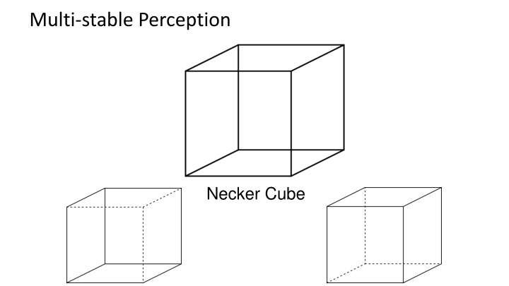
Multi-stable Perception Necker Cube
Feature Matching and Robust Fitting Read Szeliski 7.4.2 and 2.1 Computer Vision James Hays Acknowledgment: Many slides from Derek Hoiem and Grauman&Leibe 2008 AAAI Tutorial
This section: correspondence and alignment Correspondence: matching points, patches, edges, or regions across images
Review: Local Descriptors Most features can be thought of as templates, histograms (counts), or combinations The ideal descriptor should be Robust and Distinctive Compact and Efficient Most available descriptors focus on edge/gradient information Capture texture information Color rarely used K. Grauman, B. Leibe
Fitting: find the parameters of a model that best fit the data Alignment: find the parameters of the transformation that best align matched points
Fitting and Alignment Design challenges Design a suitable goodness of fit measure Similarity should reflect application goals Encode robustness to outliers and noise Design an optimization method Avoid local optima Find best parameters quickly
Fitting and Alignment: Methods Global optimization / Search for parameters Least squares fit Robust least squares Other parameter search methods Hypothesize and test Generalized Hough transform RANSAC
Fitting and Alignment: Methods Global optimization / Search for parameters Least squares fit Robust least squares Other parameter search methods Hypothesize and test Generalized Hough transform RANSAC
Least squares line fitting Data: (x1, y1), , (xn, yn) Line equation: yi = mxi + b Find (m, b) to minimize y=mx+b (xi, yi) = n = 2) ( E y m x b i i 1 i 2 1 x y 2 1 1 m m = = n 2 = = Ap y 1 E x y i i b b 1 i 1 x y n n = + T T T y y Ap y Ap Ap ( 2 ) ( ) ( ) Matlab: p = A \ y; Python: p = numpy.linalg.lstsq(A, y) dE = = T T A Ap A y 2 2 0 dp ( ) 1 = = T T T T A Ap A y p A A A y Modified from S. Lazebnik
Least squares (global) optimization Good Clearly specified objective Optimization is easy Bad May not be what you want to optimize Sensitive to outliers Bad matches, extra points Doesn t allow you to get multiple good fits Detecting multiple objects, lines, etc.
Least squares: Robustness to noise Least squares fit to the red points:
Least squares: Robustness to noise Least squares fit with an outlier: Problem: squared error heavily penalizes outliers
Fitting and Alignment: Methods Global optimization / Search for parameters Least squares fit Robust least squares Other parameter search methods Hypothesize and test Generalized Hough transform RANSAC
Robust least squares (to deal with outliers) General approach: minimize ( ( ) ) i = n , ; u x = 2 2 ( ) u y m x b i i i i 1 i ui (xi, ) residual of ith point w.r.t. model parameters robust function with scale parameter The robust function Favors a configuration with small residuals Constant penalty for large residuals Slide from S. Savarese
Choosing the scale: Just right The effect of the outlier is minimized
Choosing the scale: Too small The error value is almost the same for every point and the fit is very poor
Choosing the scale: Too large Behaves much the same as least squares
Robust estimation: Details Robust fitting is a nonlinear optimization problem that must be solved iteratively Least squares solution can be used for initialization Scale of robust function should be chosen adaptively based on median residual
Fitting and Alignment: Methods Global optimization / Search for parameters Least squares fit Robust least squares Other parameter search methods Hypothesize and test Generalized Hough transform RANSAC
Other ways to search for parameters (for when no closed form solution exists) Line search 1. For each parameter, step through values and choose value that gives best fit Repeat (1) until no parameter changes 2. Grid search 1. Propose several sets of parameters, evenly sampled in the joint set 2. Choose best (or top few) and sample joint parameters around the current best; repeat Gradient descent 1. Provide initial position (e.g., random) 2. Locally search for better parameters by following gradient
Fitting and Alignment: Methods Global optimization / Search for parameters Least squares fit Robust least squares Other parameter search methods Hypothesize and test Generalized Hough transform RANSAC
Fitting and Alignment: Methods Global optimization / Search for parameters Least squares fit Robust least squares Other parameter search methods Hypothesize and test Generalized Hough transform RANSAC
Hough Transform: Outline 1. Create a grid of parameter values 2. Each point votes for a set of parameters, incrementing those values in grid 3. Find maximum or local maxima in grid
Hough transform P.V.C. Hough, Machine Analysis of Bubble Chamber Pictures, Proc. Int. Conf. High Energy Accelerators and Instrumentation, 1959 Given a set of points, find the curve or line that explains the data points best y m b x Hough space y = m x + b Slide from S. Savarese
Hough transform y m b x y m 3 5 3 3 2 2 3 7 11 10 4 3 2 2 3 1 1 0 4 1 5 3 2 3 x b Slide from S. Savarese
Hough transform P.V.C. Hough, Machine Analysis of Bubble Chamber Pictures, Proc. Int. Conf. High Energy Accelerators and Instrumentation, 1959 Issue : parameter space [m,b] is unbounded Slide from S. Savarese
Hough transform P.V.C. Hough, Machine Analysis of Bubble Chamber Pictures, Proc. Int. Conf. High Energy Accelerators and Instrumentation, 1959 Issue : parameter space [m,b] is unbounded Use a polar representation for the parameter space y x Hough space = + x cos y sin Slide from S. Savarese
Hough transform - experiments votes features Slide from S. Savarese
Hough transform - experiments Noisy data features votes Need to adjust grid size or smooth Slide from S. Savarese
Hough transform - experiments features votes Issue: spurious peaks due to uniform noise Slide from S. Savarese
3. Hough votes Edges Find peaks and post-process
Hough transform example http://ostatic.com/files/images/ss_hough.jpg
Finding lines using Hough transform Using m,b parameterization Using r, theta parameterization Using oriented gradients Practical considerations Bin size Smoothing Finding multiple lines Finding line segments
Hough Transform How would we find circles? Of fixed radius Of unknown radius Of unknown radius but with known edge orientation
Hough transform for circles Conceptually equivalent procedure: for each (x,y,r), draw the corresponding circle in the image and compute its support r x y
Hough transform conclusions Good Robust to outliers: each point votes separately Fairly efficient (much faster than trying all sets of parameters) Provides multiple good fits Bad Some sensitivity to noise Bin size trades off between noise tolerance, precision, and speed/memory Can be hard to find sweet spot Not suitable for more than a few parameters grid size grows exponentially Common applications Line fitting (also circles, ellipses, etc.) Object instance recognition (parameters are affine transform) Object category recognition (parameters are position/scale)


 optimization")


")