Software Security Evaluation: Points to Analysis Review

Slide Note

This content covers a software security evaluation course, focusing on various analysis techniques and reviews. It includes topics such as supergraphs, interprocedural analysis, GMOD and GREF computations, and more. The discussions delve into understanding software security, evaluation methods, and enforcement needs.

sian Follow

Uploaded on Aug 14, 2024 | 1 Views

Download Presentation

Please find below an Image/Link to download the presentation.

The content on the website is provided AS IS for your information and personal use only. It may not be sold, licensed, or shared on other websites without obtaining consent from the author. Download presentation by click this link. If you encounter any issues during the download, it is possible that the publisher has removed the file from their server.

E N D

Presentation Transcript

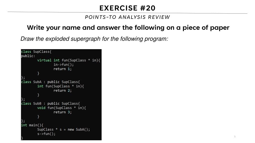
EXERCISE #20 POINTS-TO ANALYSIS REVIEW Write your name and answer the following on a piece of paper Draw the exploded supergraph for the following program: 1

ADMINISTRIVIA AND ANNOUNCEMENTS

POINTS-TO ANALYSIS EECS 677: Software Security Evaluation Drew Davidson

4 CLASS PROGRESS ANALYSIS UNDERLYING OUR ENFORCEMENT NEEDS

5 LAST TIME: INTERPROCEDURAL ANALYSIS REVIEW: LAST LECTURE CONSIDERTHEEFFECTOFMULTIPLE FUNCTIONS Simplistic Function overturn all global / aliased facts Supergraph / Context String 1-CFA (use a call-chain of 1) Summary Information - Use GMOD and GREF to cut down on imprecision

6 LAST TIME: GMOD & GREF COMPUTATION REVIEW: LAST LECTURE GLOBALS ONLY Step 1 Compute IMOD and IREF Step 2 Build (simple) call graph Step 3 Collapse Cycles Step 4 Solve a fixpoint problem Add a new exit node (and add an edge n exit for each node n with no outgoing edge. A lattice element is a set of (global) variables. The lattice meet is set union. The "initial" dataflow fact for both GMOD and GREF (the fact that holds at the exit node) is the empty set. for all nodes n, the dataflow functions for n are: GMOD: fn(S) = S U IMOD(n) GREF: fn(S) = S U IREF(n)

7 LAST TIME: GMOD & GREF COMPUTATION REVIEW: LAST LECTURE GLOBALS, LOCALS & VALUE-PASSING GREF will change, GMOD doesn t need to change Init all node GREF sets to their IREF sets Init all call site GREF sets to empty Put all nodes and call sites on a worklist Iterate until the worklist is empty. Step 1 New IREF: include locals and formals Step 2 Build call-site multigraph Step 3 Collapse Cycles Step 3 Solve a fixpoint problem Each time a node n is removed from the worklist, its current GREF set is computed. If that set doesn't match its previous value, then add all call sites to n to the worklist (if not already there). Similarly, each time a call site s is removed from the worklist, its current GREF set is computed. If that set doesn't match its previous value, then the node that contains s is added to the worklist (if not already there). GREF(n) = (U all GREF(s) s.t. s is a call site in n) U IREF(n) GREF(s) = GREF(called node m) with all formals mapped back to the corresponding actuals

8 LAST TIME: GMOD & GREF COMPUTATION REVIEW: LAST LECTURE GLOBALS, LOCALS & VALUE-PASSING GREF will change, GMOD doesn t need to change Init all node GREF sets to their IREF sets Init all call site GREF sets to empty Put all nodes and call sites on a worklist Iterate until the worklist is empty. Each time a node n is removed from the worklist, its current GREF set is computed. If that set doesn't match its previous value, then add all call sites to n to the worklist (if not present). Each time a call site s is removed from the worklist, its current GREF set is computed. If that set doesn't match its previous value, then the node that contains s is added to the worklist (if not present).

9 LAST TIME: GMOD & GREF COMPUTATION REVIEW: LAST LECTURE GLOBALS, LOCALS & VALUE-PASSING GREF will change, GMOD doesn t need to change Init all node GREF sets to their IREF sets Init all call site GREF sets to empty Put all nodes and call sites on a worklist Iterate until the worklist is empty. main IREF = { } s1 node or call site main a b s1 s2 s3 s4 GREF set g2 g2, v3, v5 f3, g2 g2 v3, g2 v5, g2 g2 void main() { S1: call a(v1) } void a( f1 ) { S2: call b(v2, v3) S3: call b(v4, v5) } void b( f2, f3 ) { print f3; S4: call b(g1, g2) } a Each time a node n is removed from the worklist, its current GREF set is computed. If that set doesn't match its previous value, then add all call sites to n to the worklist (if not present). Each time a call site s is removed from the worklist, its current GREF set is computed. If that set doesn't match its previous value, then the node that contains s is added to the worklist (if not present). IREF = { } s2 s3 b IREF = {f3} s4

10 OVERVIEW WE VE SEEN THE NECESSITY OF MULTI- FUNCTION ANALYSIS IN REAL-WORLD PROGRAMS TIME TO CONSIDER HOW IT IS DONE

11 BACK TO DATAFLOW INTERPROCEDURAL ANALYSIS What are the (possible) values of a and gbl? What is the effect of mystery on x s taintedness?

LECTURE OUTLINE May-point v Must-point Andersen s Analysis Steensgard s Analysis

13 POINTERS: LOVE TO HATE EM MAY-POINT AND MUST-POINT

14 EASY SOLUTION: DATAFLOW FOR MAY-POINT MAY-POINT AND MUST-POINT

LECTURE OUTLINE May-point v Must-point Andersen s Analysis Steensgard s Analysis

16 SUBSET CONSTRAINTS ANDERSEN S ANALYSIS A FLOW-INSENSITIVE ALGORITHM Each statement adds a constraint over the points-to sets End up with a (solvable) system of constraints Program p = &a; q = p; p = &b; r = p;

17 SUBSET CONSTRAINTS ANDERSEN S ANALYSIS

18 SUBSET CONSTRAINTS ANDERSEN S ANALYSIS A FLOW-INSENSITIVE ALGORITHM Each statement adds a constraint over the points-to sets End up with a (solvable) system of constraints Program Constraints Initial Final p = &a; q = p; p = &b; r = p; pts(p) = {a,b} pts(q) = {a,b} pts(r) = {a,b} pts(a) = pts(b) = p {a} q p p {b} r p pts(p) = pts(q) = pts(r) = pts(a) = pts(b) =

19 ANOTHER EXAMPLE ANDERSEN S ANALYSIS A FLOW-INSENSITIVE ALGORITHM Each statement adds a constraint over the points-to sets End up with a (solvable) system of constraints Program p = &a q = &b *p = q; r = &c; s = p; t = *p; *s = r; Constraints Initial pts(p) = { a } pts(q) = { b } pts(r) = { c } pts(s) = pts(t) = pts(a) = pts(b) = pts(c) = Final pts(p) = { a } pts(q) = { b } pts(r) = { c } pts(s) = { a } pts(t) = { b, c } pts(a) = { b, c } pts(b) = pts(c) = p {a} q {b} *p q r {c} s p t *p *s r

20 SOLVING CONSTRAINTS ANDERSEN S ANALYSIS Graph closure on the subset relation

21 OVERHEAD ANDERSEN S ANALYSIS WORST CASE: CUBIC TIME That s not great OPTIMIZATION: CYCLEELIMINATION Detect and collapse SCCs in the points-to relation

LECTURE OUTLINE May-point v Must-point Andersen s Analysis Steensgard s Analysis

23 AN ALTERNATIVE APPROACH STEENSGARD S ANALYSIS AIMFOR NEAR-LINEAR-TIMEPOINTS-TO ANALYSIS Going to require us to reduce our search-space somewhat INTUITION: EQUALITYCONSTRAINTS Do away with the notion of subsets