Probability Basics in Introduction to Machine Learning

Understand the concepts of random variables, probability distributions, and cumulative distribution functions in the context of machine learning. Explore examples of discrete and continuous random variables, probability mass functions, and practice problems to enhance your understanding.

• Probability Basics
• Machine Learning
• Random Variables
• Probability Distributions
• Cumulative Distribution

rubymae Follow

Uploaded on Aug 14, 2024 | 2 Views

Download Presentation

Please find below an Image/Link to download the presentation.

The content on the website is provided AS IS for your information and personal use only. It may not be sold, licensed, or shared on other websites without obtaining consent from the author.If you encounter any issues during the download, it is possible that the publisher has removed the file from their server.

You are allowed to download the files provided on this website for personal or commercial use, subject to the condition that they are used lawfully. All files are the property of their respective owners.

The content on the website is provided AS IS for your information and personal use only. It may not be sold, licensed, or shared on other websites without obtaining consent from the author.

Presentation Transcript

1. Probability Basics CS771: Introduction to Machine Learning Nisheeth

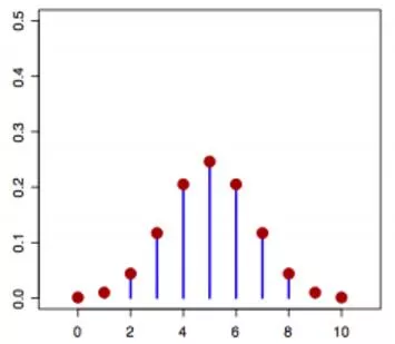
2. 2 Random Variables Informally, a random variable (r.v.) ? denotes possible outcomes of an event Can be discrete (i.e., finite many possible outcomes) or continuous Some examples of discrete r.v. ? {0,1} denoting outcomes of a coin-toss ? {1,2,...,6} denoting outcome of a dice roll ?(?) ?(a discrete r.v.) Some examples of continuous r.v. ? (0,1) denoting the bias of a coin ? denoting heights of students in CS771 ? denoting time to get to your hall from the department ?(?) ?(a continuous r.v.) CS771: Intro to ML

3. 3 Discrete Random Variables For a discrete r.v. ?, ?(?) denotes ?(? = ?) - probability that ? = ? ?(?) is called the probability mass function (PMF) of r.v. ? ?(?) or ?(? = ?) is the value of the PMF at ? ? ? 0 ? ? 1 ?(?) ?? ? = 1 ? CS771: Intro to ML

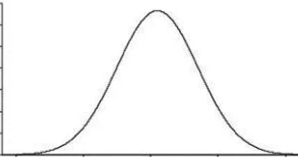
4. 4 Continuous Random Variables For a continuous r.v. ?, a probability ?(? = ?) or ?(?) is meaningless For cont. r.v., we talk in terms of prob. within an interval ? (?,? + ??) ?(?)?? is the prob. that ? (?,? + ??) as ?? 0 ?(?) is the probability density at ? = ? ? ? 0 ? ? 1 ? ? ?? = 1 CS771: Intro to ML

5. Discrete example: roll of a die p(x) 1/6 x 1 2 3 4 5 6 x all = P(x) 1 CS771: Intro to ML

6. Probability mass function (pmf) x 1 p(x) p(x=1)=1/6 2 p(x=2)=1/6 3 p(x=3)=1/6 4 p(x=4)=1/6 5 p(x=5)=1/6 6 p(x=6)=1/6 CS771: Intro to ML

7. Cumulative distribution function x 1 P(x A) P(x 1)=1/6 2 P(x 2)=2/6 3 P(x 3)=3/6 4 P(x 4)=4/6 5 P(x 5)=5/6 6 P(x 6)=6/6 CS771: Intro to ML

8. Cumulative distribution function (CDF) P(x) 1.0 5/6 2/3 1/2 1/3 1/6 x 1 2 3 4 5 6 CS771: Intro to ML

9. Practice Problem The number of patients seen in a clinic in any given hour is a random variable represented by x. The probability distribution for x is: x P(x) 10 .4 11 .2 12 .2 13 .1 14 .1 Find the probability that in a given hour: a. exactly 14 patients arrive p(x=14)= .1 p(x 12)= (.2 + .1 +.1) = .4 b. At least 12 patients arrive c. At most 11 patients arrive p(x 11)= (.4 +.2) = .6 CS771: Intro to ML

10. Continuous case The probability function that accompanies a continuous random variable is a continuous mathematical function that integrates to 1. For example, recall the negative exponential function (in probability, this is called an exponential distribution ): x = ( ) f x e This function integrates to 1: + + 0 x x = = + = 0 1 1 e e 0 CS771: Intro to ML

11. Continuous case: probability density function (pdf) p(x)=e-x 1 x The probability that x is any exact particular value (such as 1.9976) is 0; we can only assign probabilities to possible ranges of x. CS771: Intro to ML

12. For example, the probability of x falling within 1 to 2: p(x)=e-x 1 x 1 2 2 2 2 1 x x = = = = + = P(1 x 2) . 135 . 368 . 23 e e e e 1 1 CS771: Intro to ML

13. Example 2: Uniform distribution The uniform distribution: all values are equally likely. f(x)= 1 , for 1 x 0 p(x) 1 x 1 We can see it s a probability distribution because it integrates to 1 (the area under the curve is 1): 1 1 = = = 1 1 0 1 x 0 0 CS771: Intro to ML

14. Example: Uniform distribution What s the probability that x is between 0 and ? p(x) 1 x 0 1 P( x 0)= CS771: Intro to ML

15. 15 A word about notation ?(.) can mean different things depending on the context ?(?) denotes the distribution (PMF/PDF) of an r.v. ? ?(? = ?) or ??(?) or simply ?(?) denotes the prob. or prob. density at value ? Actual meaning should be clear from the context (but be careful) Exercise same care when ?(.) is a specific distribution (Bernoulli, Gaussian, etc.) The following means generating a random sample from the distribution ?(?) ? ?(?) CS771: Intro to ML

16. 16 Joint Probability Distribution Joint prob. dist. ?(?,?) models probability of co-occurrence of two r.v. ?,? For discrete r.v., the joint PMF ?(?,? ) is like a table (that sums to 1) For 3 r.v. s, we will likewise have a cube for the PMF. For more than 3 r.v. s too, similar analogy holds For two continuous r.v. s? and ?, we have joint PDF ?(?,?) For more than two r.v. s, we will likewise have a multi-dim integral for this property CS771: Intro to ML

17. 17 Marginal Probability Distribution Consider two r.v. s X and Y (discrete/continuous both need not of same type) Marg. Prob. is PMF/PDF of one r.v. accounting for all possibilities of the other r.v. For discrete r.v. s, ? ? = ??(?,? = ?) and ? ? = ??(? = ?,?) For discrete r.v. it is the sum of the PMF table along the rows/columns The definition also applied for two sets of r.v. s and marginal of one set of r.v. s is obtained by summing over all possibilities of the second set of r.v. s For discrete r.v. s, marginalization is called summing over, for continuous r.v. s, it is called integrating out For continuous r.v. s, CS771: Intro to ML

18. 18 Conditional Probability Distribution Consider two r.v. s? and ? (discrete/continuous both need not of same type) Conditional PMF/PDF ?(?|?) is the prob. dist. of one r.v. ?, fixing other r.v. ? ?(?|? = ?) or ?(? |? = ?) like taking a slice of the joint dist. ?(?,? ) Continuous Random Variables Discrete Random Variables Note: A conditional PMF/PDF may also be conditioned on something that is not the value of an r.v. but some fixed quantity in general We will see cond. dist. of output ? given weights ?(r.v.) and features ? written as ?(?|?,?) CS771: Intro to ML

19. An example X/Y raining sunny Umbrella 0.5 0.1 No umbrella 0.2 0.2 P (B|A)p(A) = p(A|B)p(B) P(x) = {0.6, 0.4} P(y) = {0.7, 0.3} P(X|Y = raining) = {0.5, 0.2} A P(A,B) B P(X = umbrella|Y = raining) CS771: Intro to ML

20. 20 Some Basic Rules Sum Rule: Sum Rule: Gives the marginal probability distribution from joint probability distribution Product Product Rule: Rule: ?(?,?) = ?(? |?)?(?) = ?(?|? )?(? ) Bayes rule: Bayes rule: Gives conditional probability distribution (can derive it from product rule) Chain Rule: Chain Rule: ?(?1,?2,...,??) = ?(?1)?(?2|?1)...?(?? |?1,...,?? 1) CS771: Intro to ML

21. 21 Independence ? and ? are independent when knowing one tells nothing about the other The above is the marginal independence (? ?) Two r.v. s? and ? may not be marginally indep but may be given the value of another r.v. ? CS771: Intro to ML

22. 22 Expectation Expectation of a random variable tells the expected or average value it takes Expectation of a discrete random variable ? ?? having PMF ?(?) Probability that ? = ? ?[?] = ??(?) ? ?? Expectation of a continuous random variable ? ?? having PDF ?(?) Probability density at ? = ? ? ? = ?? ? ?? Note that this exp. is w.r.t. the distribution ?(?(?)) of the r.v. ?(?) ? ?? Often the subscript is omitted but do keep in mind the underlying distribution The definition applies to functions of r.v. too (e.g.., ? ?(?) ) Exp. is always w.r.t. the prob. dist. ?(?) of the r.v. and often written as ??? CS771: Intro to ML

23. 23 ? and ? need not be even independent. Can be discrete or continuous Expectation: A Few Rules Expectation of sum of two r.v. s: ? ? + ? = ? ? + ?[?] Proof is as follows Define ? = ? + ? ? ? = ? ??? ?(? = ?) s.t. ? = ? + ? where ? ??and ? ?? = ? ?? ? ??(? + ?) ?(? = ?,? = ?) = ? ?? ?(? = ?,? = ?)+ ? ?? ?(? = ?,? = ?) = ?? ??(? = ?,? = ?)+ ?? ??(? = ?,? = ?) = ?? ?(? = ?)+ ?? ?(? = ?) = ? ? + ?[?] Used the rule of marginalization of joint dist. of two r.v. s CS771: Intro to ML

24. 24 Expectation: A Few Rules (Contd) ? is a real-valued scalar ? and ? are real-valued scalars Expectation of a scaled r.v.: ? ?? = ?? ? Linearity of expectation: ? ?? + ?? = ?? ? + ?? ? (More General) Lin. of exp.: ? ??(?) + ??(?) = ?? ?(?) + ?? ?(?) Exp. of product of two independent r.v. s: ? ?? = ? ? ?[?] Law of the Unconscious Statistician (LOTUS): Given an r.v. ? with a known prob. dist. ?(?) and another random variable ? = ?(?) for some function ? ? and ? are arbitrary functions. Requires only ?(?) which we already have Requires finding ?(?) = ? ? ?(?) ? ? = ? ? ? = ?? ? LOTUS also applicable for continuous r.v. s ? ?? ? ?? Rule of iterated expectation: ??(?)? = ??(?)[??(?|?)?|? ] CS771: Intro to ML

25. 25 Variance and Covariance Variance of a scalar r.v. tells us about its spread around its mean value ? ? = ? var ? = ? ? ?2= ? ?2 ?2 Standard deviation is simply the square root is variance For two scalar r.v. s? and ?, the covariance is defined by cov ?,? = ? {? ?[?]}{? ?[?]} = ? ?? ?[X]?[Y] For two vector r.v. s? and ? (assume column vec), the covariance matrix is defined by cov ?,? = ? {? ?[?]}{? ?[? ]} = ? ?? ?[X]?[? ] Cov. of components of a vector r.v. ?: cov ? = cov ?,? Note: The definitions apply to functions of r.v. too (e.g., var ?(?) ) Note: Variance of sum of independent r.v. s: var[? + ?] = var[?] + var[?] Important result CS771: Intro to ML

26. 26 Transformation of Random Variables Suppose ? = ?(?) = ?? + ? be a linear function of a vector-valued r.v. ? (? is a matrix and ? is a vector, both constants) Suppose ? ? = ? and cov ? = , then for the vector-valued r.v. ? ? ? = ? ?? + ? = ?? + ? cov ? = cov ?? + ? = ? ? Likewise, if ? = ? ? = ? ? + ? be a linear function of a vector-valued r.v. ? (? is a vector and ? is a scalar, both constants) Suppose ? ? = ? and cov ? = , then for the scalar-valued r.v. ? ? ? = ? ? ? + ? = ? ? + ? var ? = var ? ? + ? = ? ? CS771: Intro to ML

27. 27 Common Probability Distributions Important: We will use these extensively to model data as well as parameters of models Some common discrete distributions and what they can model Bernoulli: Bernoulli: Binary numbers, e.g., outcome (head/tail, 0/1) of a coin toss Binomial: Binomial: Bounded non-negative integers, e.g., # of heads in ? coin tosses Multinomial/ Multinomial/multinoulli multinoulli: : One of ? (>2) possibilities, e.g., outcome of a dice roll Poisson: Poisson: Non-negative integers, e.g., # of words in a document Some common continuous distributions and what they can model Uniform: Uniform: numbers defined over a fixed range Beta: Beta: numbers between 0 and 1, e.g., probability of head for a biased coin Gamma: Gamma: Positive unbounded real numbers Dirichlet: Dirichlet: vectors that sum of 1 (fraction of data points in different clusters) Gaussian: Gaussian: real-valued numbers or real-valued vectors CS771: Intro to ML