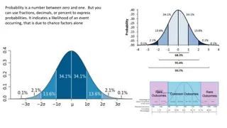
Understanding Probability Concepts in "The Mathematics of Star Trek Workshop
Explore the intriguing topic of probability through the lens of the popular culture reference to Red Shirts in Star Trek. Delve into basic probability concepts, sample spaces, and experiments, illustrated with interesting examples.

Download Presentation

Please find below an Image/Link to download the presentation.
The content on the website is provided AS IS for your information and personal use only. It may not be sold, licensed, or shared on other websites without obtaining consent from the author. Download presentation by click this link. If you encounter any issues during the download, it is possible that the publisher has removed the file from their server.
E N D
Presentation Transcript
The Mathematics of Star Trek Workshop Lecture 1: Red Shirt Survivability
Red Shirts in Star Trek TOS Two terms that have entered popular culture are red shirt and expendable crewmember. In Star Trek TOS, often the crew member(s) wearing a red shirt as part of their uniform die soon after being introduced. A natural question to ask is what is the likelihood of dying in the Star Trek Universe if one s uniform is red? 2
Outline Basic Probability Concepts Star Trek TOS Data Conditional Probability Answer the Question! 3
Basic Probability Concepts Formally, the study of probability began with the posthumous publication of Girolamo Cardano s Book on Games and Chance in 1663. Probably he wrote it in ~1563. Other key players in the development of this branch of mathematics include: Blaise Pascal and Pierre de Fermat (17th century). Jakob Bernoulli (late 17th century). 4
Definition of Probability One way to define probability is as follows: The probability of an event E is a quantified assessment of the likelihood of E. By quantified, we mean a number is assigned. In order to understand this definition, we need some more definitions and concepts! 5
More Definitions! Each time we consider a probability problem, we think of it as an experiment, either real or imagined. An experiment is a test or trial of something that is repeatable. The first step in such a problem is to consider the sample space. The sample spaceS of an experiment is a set whose elements are all the possible outcomes of the experiment. 6
Example 1: Some Experiments and Sample Spaces 1(a) Experiment: Select a card from a deck of 52 cards. Sample Space: S = {A , A , A , A , 2 , 2 , 2 , 2 , K , K , K , K } 1(b) Experiment: Poll a group of voters on their choice in an election with three candidates, A, B, and C. Sample Space: S = { A, B, C}. 7
Example 1: Some Experiments and Sample Spaces (cont.) 1(c) Experiment: Flip a coin, observe the up face. Sample Space: S = {H, T} 1(d) Experiment: Roll two six-sided dice, observe up faces. Sample Space: S = {(1,1), (1,2), (1,3), (1,4), (1,5), (1,6), , (6,1), (6,2), (6,3), (6,4), (6,5), (6,6)} 8
Another Definition! When working with probability, we also need to define event. An event E is any subset of the sample space S. An event consists of any number of outcomes in the sample space. Notation: E S. 9
Example 2: Some Events 2(a) Experiment: Select a card from a deck of 52 cards. Sample Space: S = {A , A , A , A , 2 , 2 , 2 , 2 , K , K , K , K } Event: Select a card with a diamond. E = {A , 2 , , K } 10
Example 2: Some Events (cont.) 2(b) Experiment: Poll a group of voters on their choice in an election with three candidates, A, B, and C. Sample Space: S = { A, B, C} Event: Voter chooses B or C. E = {B,C}. 11
Example 2: Some Events (cont.) 2(c) Experiment: Flip a coin, observe the up face. Sample Space: S = {H, T} Event: Up face is Tail. E = {T}. 12
Example 2: Some Events (cont.) 2(d) Experiment: Roll two six-sided dice, observe up faces. Sample Space: S = {(1,1), (1,2), (1,3), (1,4), (1,5), (1,6), , (6,1), (6,2), (6,3), (6,4), (6,5), (6,6)} Event: Roll a pair: E = {(1,1}, (2,2), (3,3), (4,4), (5,5), (6,6)} 13
Example 2: Some Events (cont.) 2(e) Experiment: Roll two six-sided dice, add the up faces. Sample Space: S = {2, 3, 4, 5, 6, 7, 8, 9, 10, 11, 12} Event: Roll an odd sum: E = {3, 5, 7, 9, 11} 14
Probability of an Event With these definitions, we can now define how to compute the probability of an event! 15
How to find the Probability of an Event E Determine the elements of the sample space S. S = {s1, s2, , sn}. Assign a weight or probability (i.e. number) to each element of S in such a way that: Each weight is at least 0 and at most 1. The sum of all the weights is 1. (For each element si in S, denote its weight by p(si).) Add the weights of all outcomes contained in event E. The sum of the weights of E is the probability of E and is denoted p(E). 1. 2. 3. 4. 16
How to find the Probability of an Event E (cont.) Notes: Weights may be assigned in any fashion in Step 2, as long as both conditions are met. Usually we choose weights that make sense in reality. A probability model is a sample space S together with probabilities for each element of S. If each element of sample space S has the same probability, the model is said to have equally likely outcomes. 17
Example 3: Some Probability Models 3(a) Experiment: Select a card from a deck of 52 cards. Sample Space: S = {A , A , A , A , 2 , 2 , 2 , 2 , K , K , K , K } p(A ) = p(A ) = = p(K ) = p(K ) = 1/52 For the event select a card with a diamond , E = {A , 2 , , K } and p(E) = p(A ) + p(2 ) + + p(K ) = 13/52 = 1/4. 18
Example 3: Some Probability Models (cont.) 3(b) Experiment: Poll a group of voters on their choice in an election with three candidates, A, B, and C. Sample Space: S = { A, B, C} p(A) = 0.42; p(B) = 0.15; p(C) = 0.43. For the event a voter chooses B or C , E = {B,C} and p(E) = p(B) + p(C) = 0.15 + 0.43 = 0.58. 19
Example 3: Some Probability Models (cont.) 3(c) Experiment: Flip a coin, observe the up face. Sample Space: S = {H, T} p(H) = 1/2; p(T) = 1/2 For the event the up face is Tail , E = {T} and p(E) = 1/2. 20
Example 3: Some Probability Models (cont.) 3(d) Experiment: Roll two six-sided dice, observe up faces. Sample Space: S = {(1,1), (1,2), (1,3), (1,4), (1,5), (1,6), , (6,1), (6,2), (6,3), (6,4), (6,5), (6,6)} p((i,j)) = 1/36 for each i = 1,2, , 6; j = 1, 2, , 6. For the event roll a pair , E = {(1,1}, (2,2), (3,3), (4,4), (5,5), (6,6)}, so p(E) = 1/36 + 1/36 + +1/36 = 6/36 = 1/6. 21
Example 3: Some Probability Models (cont.) 3(e) Experiment: Roll two six-sided dice, add the up faces. Sample Space: S = {different possible sums} = {2, 3, 4, 5, 6, 7, 8, 9, 10, 11, 12} Using the probability model for example 3 (d), we find p(2) = 1/36; p(3) = 2/36; p(4) = 3/36; p(5) = 4/36; p(6) = 5/36; p(7) = 6/36; p(8) = 5/36; p(9) = 4/36; p(10) = 3/36; p(11) = 2/36; p(12) = 1/36. For the event roll an odd sum , E = {3, 5, 7, 9, 11} and p(E) = p(3) + p(5) + p(7) + p(9) + p(11) = 2/36 + 4/36 + 6/36 + 4/36 + 2/36 = 18/36 = 1/2. 22
Remark on Probability Models with Equally Likely Outcomes Examples 3(a), 3(c), and 3(d) are probability models with equally likely outcomes. Notice that in each case, p(E) = (# elements in E)/(# elements in S). This is true in general for probability models with equally likely outcomes! Notice that this property fails for examples 3(b) and 3(e). For example, in 3(e), # elements in E = 5 and # elements in S = 11, but p(E) = 1/2. 23
Back to the Star Trek Universe! Now we are ready to look at some Star Trek Examples! Of the 43 on- screen deaths in TOS, 10 were gold shirts, 8 were blue shirts, and 25 were red shirts. 8 25 10 24
Example 4 Assuming all on-screen deaths are equally likely, what would be the probability that a crew member who died has a red shirt? Solution: S = {crew members that died} E = {red shirt} P(E) = (# E)/(# S) = 25/43 = 58.1% 8 25 10 25
Example 4 (cont.) Similarly, we find that the probabilities that a crew member who died onscreen is wearing a gold shirt or blue shirt are: 10/43 = 23.3% and 8/43 = 18.6%, respectively. 8 25 10 26
Conditional Probability So, have we answered the question: What is the likelihood of dying if a crew member s shirt is red? No actually, in Example 4 we have answered the question: What is the likelihood of a crew member s shirt being red if the crew member dies? The answer to each of these questions involves the idea of conditional probability. 27
Conditional Probability Suppose for some experiment we are interested only in those outcomes that are elements of a subset of the sample space. Then we can think of the subset as our sample space and use the ideas above to find probabilities of events from this subset! We can think of the last example in these terms 28
Conditional Probability Assume all crew members of the Starship Enterprise have an equal chance of being chosen. Think of the crew members who die as a subset of the entire crew. Let A = {red shirts} and B = {crew members who die}. From Example 4, the probability that a crew member who dies has a red shirt is (# red shirts who die)/(# crew members who die) = (# in A and B)/(# in B) = 25/43 If we divide both numerator and denominator by the total number of crew members, then we can write this last ratio as 25/43 = (25/430)/(43/430) =((# in A and B)/total # crew)/ ((# in B)/(total # crew)) =P(A B)/P(B) Starship Enterprise Crew Data Uniform Color Fatalities Gold 10 Blue 8 Red 25 Total 43 Known Total Population 55 136 239 430 29
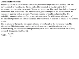
Conditional Probability Examples like this last one are the basis for the following definition. The conditional probability of an event A given that event B has occurred is defined by P(A|B) = P(A B)/P(B). Note that P(B) > 0 for this definition to make sense. 30
Finally the Answer! Now we are ready to answer the question What is the likelihood of dying if a crew member s shirt is red? i.e. What is the probability that a crew member dies given that the crew member is wearing a red shirt? Let A = {crew members who die} and B = {red shirts}. What we want to find is the conditional probability P(A|B). P(A|B) = P(A B)/P(B) = (25/430)/(239/430) = 25/239 = 10.5% Note that this is also (# red shirt deaths)/(# red shirts) Starship Enterprise Crew Data Uniform Color Fatalities Gold 10 Blue 8 Red 25 Total 43 Known Total Population 55 136 239 430 31
The Safest Shirt Color! Similarly, one finds that the probability that a crew member with a gold shirt dies is 18.2%, and the probability that a crew member with a blue shirt dies is 5.9%. Thus, the least safe shirt color is actually GOLD!! Starship Enterprise Crew Data Uniform Color Fatalities Gold 10 Blue 8 Red 25 Total 43 Known Total Population 55 136 239 430 32
References For All Practical Purposes (5th ed.) by COMAP The Cartoon Guide to Statistics by Gonick and Smith Probability and Statistical Inference (5th ed.) by Hogg and Tanis http://aperiodical.com/2013/04/the-maths- of-star-trek-the-original-series-part-i/ 33


")