Introduction to Machine Learning in BMTRY790 Course

 
Lecture 1: Overview of Machine
Learning
 
BMTRY 790: Machine Learning
 
General Information
 
Website
:
http://people.musc.edu/~wolfb/BMTRY790_Spring2023/BMTRY790_2023.htm
Office
: 302B, 135 Cannon Place
Phone
: (843)876-1940
Email
: wolfb@musc.edu
Office Hours
: By appointment
 
Homework
 
4-5 homework assignments worth 60% of your
grade.
Include some theory, application of software, as well as
writing your own code.
Should be submitted electronically.  Scan hand-written
homework send electronic copy.
Due 1 week after it is assigned unless otherwise noted.
One day late will receive a 25% reduction, two days late
will receive a 50% reduction, more than two days late will
not be accepted.
 
Exam
 
There will also be one mid-term exam that
constitutes 20% of your grade.
 
The exam will consist  of:
Theory of statistical learning algorithms
Writing pseudo code for programming statistical
algorithms
Comparison of different statistical learning algorithms.
 
Project
 
Designed to simulate a real problem you may face
once you’ve graduate- how to choose from among
different modeling techniques.
 
The goal will be to use the methods learned
throughout the class to develop a prediction model
for real-world data.
 
What is Machine Learning
 
Making computers adapt or modify their actions to
lead to a more accurate actions…
 
Examples of actions
Predicting a patient’s response
Identifying subsets of similar observations
Extraction of features relevant to an outcome
 
Types of Machine Learning
 
Supervised
Have a set of training of observations with both
predictors and response(s)
 
Unsupervised
Have a set of features but no response is provided
Goal is to identify similar observations
 
Types of Machine Learning
 
Reinforcement
Between supervised and unsupervised
Algorithm told when it is right or wrong
“Rewarded” for correct action
“Penalized” for mistakes
Examples include things like teaching a computer
to play a game
i.e. what is the best move to make at this time?
 
Vocabulary: Statistics vs. ML
 
Dependent Variable (
Y
, 
G
, 
t
)
Response
Outcome
Target
Output
Independent Variables (
X
)
Predictors
Features
Inputs
 
Goal In Machine Learning
 
General goal
discover patterns in data through the use of algorithms
use these patterns to take some action
 
Examples?


Goal In Machine Learning
 
In a more mathematical/statistical context
Given input features 
x
Find a function 
f 
(
x
)
 that does a good job of
predicting/estimating an outcome 
y
 
Linear regression is an example of this


Ideally we want the results from our learner to be
generalizable
 
Simple Example
 
We want to understand bioavailability of iron in
rainwater to phytoplankton
Iron is a limiting nutrient and certain “forms” of iron are
more available for phytoplankton to use
Ionic iron (Fe
2+
 or Fe
3+
) are more available than colloidal
iron (e.g. Fe
2
O
3 
= rust).
Major source of iron in the open ocean is from rainwater
We want to evaluate if there is a relationship between
time of day with Fe
3+
 
Simple Example
 
We observe some real-valued input variable 
x
 = time
for 10 rain events and we want to predict 
y
 
= Fe
3+
 
This is a problem we are familiar with…  What is one
approach we might take?
 
Simple Example
 
Let’s say we run a regression model
 
Polynomial Fits
 
Coefficients with Increasing Order
 
y 
=
 f(x) 
=
 sin
(2
x
) + 
 
 
Polynomial Fits
 
Examining Overfitting
 
What about with more data?
 
Impact of Larger 
N
 on Overfitting
 
 
Another Simple Example
 
Consider an example where we have a data set with
2 features 
x
1
 and 
x
2
 and an output variable, 
y
, with
two classes
e.g. classify Cooper River Bridge run participants as
runners/walkers based on chip time and age
 
We want to develop a prediction rule for determining
the class of 
y
 
based on 
x
1
 
and
 
x
2
i.e. find some                   yields a good prediction
 
 
What methods might we use that we know already?
 
“Linear” Regression Approaches
 
We could simply develop a linear model
 
How can we use the output to classify 
y
 and develop
a decision boundary?
 
“Linear” Regression Approaches
 
Decision boundary from linear regression model


“Linear” Regression Approaches
 
Alternatively we could use a link function
i.e. logistic regression
 
How can this type of mode be used to develop a
decision boundary
 
“Linear” Regression Approaches
 
Decision boundary from logistic regression model


Linear Classifiers
 
Caveats
 
Linear classifiers yield relatively stable predictions
 
However, we make relatively large assumptions
about the association between 
y
 and our features 
x
Classes are linearly separable
Inputs/predictors are independent
Independence of errors
 
There are (many?) times when these assumptions
are unreasonable
 
Alternatives
 
The regression approaches are model based and
assume a specific relationship between 
X
 and 
Y
 
There are many alternatives to traditional linear
regression classifiers
 
Here we briefly examine 1…  nearest neighbors
 
Nearest Neighbors
 
Idea
:  use the 
k
 observations closest to point 
x
i
 to
develop a decision boundary to determine the
predicted class
Mathematically we can express this as follows
 
 
There are certainly fewer assumptions but what
assumption does this still make?
 
K-Nearest Neighbors
 
Caveats for kNN
 
Requires fewer assumptions and can adapt to any
scenario
 
However, sub-regions of the decision boundary are
determined by only a small subset of the training
observations
Results is that kNN often produced unstable estimates
 
Loss Functions
 
In trying to define 
f 
(
X
)
 to predict 
Y
 given our
values of 
X
, we need to choose a loss function
to penalize prediction errors.
 
Familiar loss functions
 
Loss Functions
 
Selecting the loss function leads us to a
criterion for choosing
Goal is to minimize the expected loss
 
Least Squares Example
 
In Context of LR and kNN?
 
Thus for regression our best estimation of 
Y
 when
X
=
x
 is the conditional mean of 
Y
 at 
X=x.
 
The NN approach directly implements this idea in
local regions in the training data
 
Expectation approximated by average all 
y
i
’s in the
neighborhood of 
X=x
 
 
Conditioning on relaxed region close to observation 
X=x
 
 
Curse of Dimensionality
 
Refers to problems with analyzing high-dimensional
data that do not occur in low-dimensional settings.
 
As the number of features increases, the feature
space volume increases so fast that the data become
sparse.
Result is that our intuition breaks down as dimensions
increase.
 
Curse of Dimensionality
 
If evaluating statistical significance, the amount of
data needed to support the result often grows
exponentially with the dimensionality
 
For discovery (i.e. discover patterns), organizing and
searching the  data relies on detecting areas where
objects form groups with similar properties
In high dimensional data, all objects may appear to be
sparse, which prevents common data organization
strategies from being efficient
 
Consider Our Examples
 
Polynomial fit
We considered a case with only a single variable
But what happens if we consider 
D
 variables?
 
Consider Our Examples
 
k
-NN:
We considered a case with two variables
Consider two classed based on 
D
 inputs uniformly
dispersed in a 
D
-dimensional hypercube of unit volume
Want capture hypercubical neighborhood around a target point to
capture a fraction 
r 
of the unit volume
Expected edge length is 
e
D
(
r
) = 
r
1/
D
In 10 dimensions for 
r
 = 0.1 
this means 
e
10
(0.1) = 0.80
However, the range of each input is only 1.0
 
More on Supervised Learning
 
Start with assumptions that data come from a model
Y
 = 
f
(
x
) + 
 where 
E
(
) = 0 
and is independent of 
X
 
Here 
f
(
x
) = 
E
(
Y
|
X
 = 
x
)
 
Goal of supervised learning is to learn 
f
  by example
 
Learning algorithm can modify the input/output
relationship     based on
 
Function Approximation
 
Data 
{
x
i
, 
y
i
} 
considered 
(
p
+1)-
dim Euclidean space
 
f
(
x
)
 has domain of p-dim input space and is related
to data via a model like 
y
i
 = 
f
(
x
i
) + 
 
Goal to obtain useful approximation for 
f
(
x
)
 based on
all 
x
Many approximations include estimated set of
parameters 
Linear regression: 
f
(
x
) = 
x
   
 
 = 
More general:                                      (linear basis expansion)
 
On Writing R Functions…
 
Idea:
Objects created within a function are local to the
environment of the function
They don’t exist outside of the function.
But you can “return” a value(s) of the object from
the function
Can be used in other functions
Can summarize results of task the function completed
 
Why Write Your Own Functions?
 
Easy way to conduct simulations for method
evaluation
 
Standardize code you use often
Once function written, need one line of code to run your
analysis
e.g. plotting functions to summarize results
 
Developing and disseminating new methods
 
Basic Function Format
 
Need a function name
Arguments (generally at least)
Body of code that does some task
Final object the function returns (not
necessary)
 
Pseudo Code- Simple Example
 
What do we need to generate our data sin(x) example
 
y 
=
 f(x) 
=
 sin
(2
x
) + 
 
 
Pseudo Code- Simple Example
 
What do we need to generate our data sin(x) example
 
Code for Simple Example
 
 
polyfit<-function(dat, maxpol)
{
 models<-vector("list", maxpol+1)
 prd<-matrix(0, nrow=nrow(nxs), ncol=maxpol)
 tst<-myfunc(100)
 prdtrn<-errtrn<-matrix(0, nrow=nrow(dat), ncol=maxpol)
 prdnew<-errnew<-matrix(0, nrow=100, ncol=maxpol)
 model.basis<-lm(y ~ 1, dat)
 models[[1]]<-model.basis$coef
 for (i in 1:maxpol)
 
{
 
modi<-lm(y ~ poly(x, i, raw=TRUE), data=dat)
 
models[[i+1]]<-modi$coef
 
prdtrn[,i]<-predict(modi)
 
errtrn[,i]<-(prdtrn[,i]-dat$y)^2
 
prdnew[,i]<-predict(modi, newdata=tst[,2])
 
errnew[,i]<-(prdnew[,i]-tst$y[1:94])^2
 
}
 ans<-list(models=models, ptrn=prdtrn, etrn=errtrn, pnew=prdnew, enew=errnew)
 return(ans)
}
 
More Complex Example
 
Troubleshooting
 
R and Rstudio do have a debug() function
 
Use print statements to determine when code breaks
 
Use toy examples for which you know how the
output should look and can compare what your
function returns with what it should return
 
Comment code to help yourself as well!
 
Examples of Trouble Shooting
 
Using print statements to understand an error
 
Goal
: Develop a function to calculate the odds ratios
for all possible cut-points for a single continuous
variable 
x
 and a categorical variable 
y
 
Understanding Error Message
 
calcOR_allX<-function (x, y) {
    ORs<-c()
    for (i in 1:length(x))
 
{
 
cp<-sort(x)[i]
 
Ix<-ifelse(x>cp, 1, 0)
 
tab<-table(Ix, y)
 
ORs<-append(ORs, (tab[1,1]*tab[2,2])/(tab[1,2]*tab[2,1]))
 
}
   return(ORs)
}
 
> calcOR_allX(x=x, y=y)
Error in tab[2, 2] : subscript out of bounds
 
Understanding Error Message
 
calcOR_allX<-function (x, y) {
    ORs<-c()
    for (i in 1:length(x))
 
{
 
cp<-sort(x)[i]
 
Ix<-ifelse(x>cp, 1, 0)
 
tab<-table(Ix, y)
  print(paste("Table for cut-point", i,sep=" "))
  print(tab)
 
ORs<-append(ORs, (tab[1,1]*tab[2,2])/(tab[1,2]*tab[2,1]))
 
}
   return(ORs)
}
calcOR_allX(x=x, y=y)
[1] "Table for cut-point 100"
   y
Ix   0  1
  0 50 50
Error in tab[2, 2] : subscript out of bounds
 
Understanding Error Message
 
calcOR_allX<-function (x, y) {
    ORs<-c()
    for (i in 1:length(x))
 
{
 
cp<-sort(x)[i]
 
Ix<-ifelse(x>cp, 1, 0)
 
tab<-table(Ix, y)
 
if (dim(tab)[1]==dim(tab)[2])
  
{ORs<-append(ORs, (tab[1,1]*tab[2,2])/(tab[1,2]*tab[2,1]))}
 
}
   return(ORs)
}
>tst<- calcOR_allX(x=x, y=y)
>tst
[1]      Inf      ...
[97] 2.041667 1.000000      Inf
 
Examples of Trouble Shooting
 
Using toy examples to check your code
 
Goal
: Develop a function to calculate the relative risk
for a binary variable 
x
 and a categorical variable 
y
 
Test Examples
 
calcRR<-function (x, y) {
   tab<-table(x, y)
   if (dim(tab)[1]==dim(tab)[2])
 
{  RR<-(tab[1,1]/sum(tab[,1]))/(tab[2,1]/sum(tab[2,]))  }
   return(RR)
}
>dat
        x   y
 [1,] 1   0
 [2,] 1   0
 [3,] 0   1
 [4,] 1   0
 [5,] 1   0
 [6,] 0   1
 [7,] 1   1
 [8,] 0   0
 [9,] 1   0
[10,] 1  0
>calcRR(x=dat$x, y=dat$y)
[1] 0.1667
 
Test Examples
 
calcRR<-function (x, y) {
   tab<-table(x, y)
   print("This is the 2x2 table")
   print(tab)
   if (dim(tab)[1]==dim(tab)[2])
 
{  RR<-(tab[1,1]/sum(tab[,1]))/(tab[2,1]/sum(tab[2,]))  }
   return(RR)
}
>calcRR(x=dat$x, y=dat$y)
[1] "This is the 2x2 table"
       y
x     0   1
  0   1   2
  1   6   1
[1] 0.1666667
 
Test Examples
 
calcRR<-function (x, y) {
   tab<-table(x, y)
   print("This is the 2x2 table")
   print(tab)
   if (dim(tab)[1]==dim(tab)[2])
 
{  RR<-(tab[2,2]/sum(tab[,2]))/(tab[1,2]/sum(tab[1,]))  }
   return(RR)
}
 
>calcRR(x=dat$x, y=dat$y)
[1] "This is the 2x2 table"
       y
x     0   1
  0   1   2
  1   6   1
[1] 0.5
 
Test Examples
 
calcRR<-function (x, y) {
   tab<-table(x, y)
   print("This is the 2x2 table")
   print(tab)
   if (dim(tab)[1]==dim(tab)[2])
 
{  RR<-(tab[2,2]/sum(tab[2,]))/(tab[1,2]/sum(tab[1,]))  }
   return(RR)
}
 
>calcRR(x=dat$x, y=dat$y)
[1] "This is the 2x2 table"
       y
x     0   1
  0   1   2
  1   6   1
[1] 0.2143
 
Next Time
 
Review simple and multiple regression (this is
a lead into variable selection techniques and
adaptations to linear regression models)
Slide Note
Embed
Share

The BMTRY790 course on Machine Learning covers a wide range of topics including supervised, unsupervised, and reinforcement learning. The course includes homework assignments, exams, and a real-world project to apply learned methods in developing prediction models. Machine learning involves making computers adapt their actions for accurate predictions. Supervised learning uses training data with predictors and responses, unsupervised learning identifies similar observations, and reinforcement learning teaches algorithms through rewards and penalties. Visit the course website for more details.

  • Machine Learning
  • BMTRY790
  • Supervised Learning
  • Unsupervised Learning
  • Reinforcement Learning

Uploaded on Sep 21, 2024 | 2 Views


Download Presentation

Please find below an Image/Link to download the presentation.

The content on the website is provided AS IS for your information and personal use only. It may not be sold, licensed, or shared on other websites without obtaining consent from the author. Download presentation by click this link. If you encounter any issues during the download, it is possible that the publisher has removed the file from their server.

E N D

Presentation Transcript


  1. Lecture 1: Overview of Machine Learning BMTRY 790: Machine Learning

  2. General Information Website: http://people.musc.edu/~wolfb/BMTRY790_Spring2023/BMTRY790_2023.htm Office: 302B, 135 Cannon Place Phone: (843)876-1940 Email: wolfb@musc.edu Office Hours: By appointment

  3. Homework 4-5 homework assignments worth 60% of your grade. Include some theory, application of software, as well as writing your own code. Should be submitted electronically. Scan hand-written homework send electronic copy. Due 1 week after it is assigned unless otherwise noted. One day late will receive a 25% reduction, two days late will receive a 50% reduction, more than two days late will not be accepted.

  4. Exam There will also be one mid-term exam that constitutes 20% of your grade. The exam will consist of: Theory of statistical learning algorithms Writing pseudo code for programming statistical algorithms Comparison of different statistical learning algorithms.

  5. Project Designed to simulate a real problem you may face once you ve graduate- how to choose from among different modeling techniques. The goal will be to use the methods learned throughout the class to develop a prediction model for real-world data.

  6. What is Machine Learning Making computers adapt or modify their actions to lead to a more accurate actions Examples of actions Predicting a patient s response Identifying subsets of similar observations Extraction of features relevant to an outcome

  7. Types of Machine Learning Supervised Have a set of training of observations with both predictors and response(s) Unsupervised Have a set of features but no response is provided Goal is to identify similar observations

  8. Types of Machine Learning Reinforcement Between supervised and unsupervised Algorithm told when it is right or wrong Rewarded for correct action Penalized for mistakes Examples include things like teaching a computer to play a game i.e. what is the best move to make at this time?

  9. Vocabulary: Statistics vs. ML Dependent Variable (Y, G, t) Response Outcome Target Output Independent Variables (X) Predictors Features Inputs

  10. Goal In Machine Learning General goal discover patterns in data through the use of algorithms use these patterns to take some action Examples?

  11. Goal In Machine Learning In a more mathematical/statistical context Given input features x Find a function f (x) that does a good job of predicting/estimating an outcome y Linear regression is an example of this ( ) f x = = x ' y Ideally we want the results from our learner to be generalizable

  12. Simple Example We want to understand bioavailability of iron in rainwater to phytoplankton Iron is a limiting nutrient and certain forms of iron are more available for phytoplankton to use Ionic iron (Fe2+or Fe3+) are more available than colloidal iron (e.g. Fe2O3 = rust). Major source of iron in the open ocean is from rainwater We want to evaluate if there is a relationship between time of day with Fe3+

  13. Simple Example We observe some real-valued input variable x = time for 10 rain events and we want to predict y = Fe3+ This is a problem we are familiar with What is one approach we might take?

  14. Simple Example Let s say we run a regression model

  15. Polynomial Fits

  16. Coefficients with Increasing Order M=0 M=1 M=3 M=6 M=9 b0 -0.112 0.721 -0.014 0.052 0.068 b1 -1.852 8.692 2.564 -16.590 b2 -27.218 38.797 244.86 b3 18.504 -258.484 693.33 b4 555.678 -19609.9 b5 -533.186 102882.1 b6 196.115 -257122.5 b7 343211.3 b8 -235721.8 b9 65522.27

  17. y = f(x) = sin(2x) +

  18. Polynomial Fits

  19. Examining Overfitting

  20. What about with more data?

  21. Impact of Larger N on Overfitting

  22. Another Simple Example Consider an example where we have a data set with 2 features x1and x2and an output variable, y, with two classes e.g. classify Cooper River Bridge run participants as runners/walkers based on chip time and age We want to develop a prediction rule for determining the class of y based on x1and x2 i.e. find some yields a good prediction ( ) y f x = What methods might we use that we know already?

  23. Linear Regression Approaches We could simply develop a linear model How can we use the output to classify y and develop a decision boundary?

  24. Linear Regression Approaches Decision boundary from linear regression model

  25. Linear Regression Approaches Alternatively we could use a link function i.e. logistic regression How can this type of mode be used to develop a decision boundary

  26. Linear Regression Approaches Decision boundary from logistic regression model

  27. Linear Classifiers

  28. Caveats Linear classifiers yield relatively stable predictions However, we make relatively large assumptions about the association between y and our features x Classes are linearly separable Inputs/predictors are independent Independence of errors There are (many?) times when these assumptions are unreasonable

  29. Alternatives The regression approaches are model based and assume a specific relationship between X and Y There are many alternatives to traditional linear regression classifiers Here we briefly examine 1 nearest neighbors

  30. Nearest Neighbors Idea: use the k observations closest to point xito develop a decision boundary to determine the predicted class Mathematically we can express this as follows 1 k ( ) = Y x y i ( ) x x N i k There are certainly fewer assumptions but what assumption does this still make?

  31. K-Nearest Neighbors

  32. Caveats for kNN Requires fewer assumptions and can adapt to any scenario However, sub-regions of the decision boundary are determined by only a small subset of the training observations Results is that kNN often produced unstable estimates

  33. Loss Functions In trying to define f (X) to predict Y given our values of X, we need to choose a loss function to penalize prediction errors. Familiar loss functions squared error loss: absolute error loss: zero one loss

  34. Loss Functions Selecting the loss function leads us to a criterion for choosing Goal is to minimize the expected loss

  35. Least Squares Example

  36. In Context of LR and kNN? Thus for regression our best estimation of Y when X=x is the conditional mean of Y at X=x. The NN approach directly implements this idea in local regions in the training data Expectation approximated by average all yi s in the neighborhood of X=x ( ) ( Ave i f x y x ) ( ) x = N i k Conditioning on relaxed region close to observation X=x

  37. Curse of Dimensionality Refers to problems with analyzing high-dimensional data that do not occur in low-dimensional settings. As the number of features increases, the feature space volume increases so fast that the data become sparse. Result is that our intuition breaks down as dimensions increase.

  38. Curse of Dimensionality If evaluating statistical significance, the amount of data needed to support the result often grows exponentially with the dimensionality For discovery (i.e. discover patterns), organizing and searching the data relies on detecting areas where objects form groups with similar properties In high dimensional data, all objects may appear to be sparse, which prevents common data organization strategies from being efficient

  39. Consider Our Examples Polynomial fit We considered a case with only a single variable But what happens if we consider D variables? ( ) f x D D D D D D = = + + + + y ... x x x x x x 0 j j jk j k jkl j k l = = = = = = 1 1 1 1 1 1 j j k j k l M For an -order polynomial, the growth of the coefficients is proportional to M D

  40. Consider Our Examples k-NN: We considered a case with two variables Consider two classed based on D inputs uniformly dispersed in a D-dimensional hypercube of unit volume Want capture hypercubical neighborhood around a target point to capture a fraction r of the unit volume Expected edge length is eD(r) = r1/D In 10 dimensions for r = 0.1 this means e10(0.1) = 0.80 However, the range of each input is only 1.0

  41. More on Supervised Learning Start with assumptions that data come from a model Y = f(x) + where E( ) = 0 and is independent of X Here f(x) = E(Y|X = x) Goal of supervised learning is to learn f by example Learning algorithm can modify the input/output relationship based on f ( ) f x y i i

  42. Function Approximation Data {xi, yi} considered (p+1)-dim Euclidean space f(x) has domain of p-dim input space and is related to data via a model like yi = f(xi) + Goal to obtain useful approximation for f(x) based on all x Many approximations include estimated set of parameters Linear regression: f(x) = x = More general: (linear basis expansion) ( ) 1 k f x = = ( ) x K h k k

  43. On Writing R Functions Idea: Objects created within a function are local to the environment of the function They don t exist outside of the function. But you can return a value(s) of the object from the function Can be used in other functions Can summarize results of task the function completed

  44. Why Write Your Own Functions? Easy way to conduct simulations for method evaluation Standardize code you use often Once function written, need one line of code to run your analysis e.g. plotting functions to summarize results Developing and disseminating new methods

  45. Basic Function Format Need a function name Arguments (generally at least) Body of code that does some task Final object the function returns (not necessary)

  46. Pseudo Code- Simple Example What do we need to generate our data sin(x) example

  47. y = f(x) = sin(2x) +

  48. Pseudo Code- Simple Example What do we need to generate our data sin(x) example

  49. Code for Simple Example

  50. More Complex Example polyfit<-function(dat, maxpol) { models<-vector("list", maxpol+1) prd<-matrix(0, nrow=nrow(nxs), ncol=maxpol) tst<-myfunc(100) prdtrn<-errtrn<-matrix(0, nrow=nrow(dat), ncol=maxpol) prdnew<-errnew<-matrix(0, nrow=100, ncol=maxpol) model.basis<-lm(y ~ 1, dat) models[[1]]<-model.basis$coef for (i in 1:maxpol) { modi<-lm(y ~ poly(x, i, raw=TRUE), data=dat) models[[i+1]]<-modi$coef prdtrn[,i]<-predict(modi) errtrn[,i]<-(prdtrn[,i]-dat$y)^2 prdnew[,i]<-predict(modi, newdata=tst[,2]) errnew[,i]<-(prdnew[,i]-tst$y[1:94])^2 } ans<-list(models=models, ptrn=prdtrn, etrn=errtrn, pnew=prdnew, enew=errnew) return(ans) }

More Related Content

giItT1WQy@!-/#giItT1WQy@!-/#giItT1WQy@!-/#giItT1WQy@!-/#giItT1WQy@!-/#giItT1WQy@!-/#giItT1WQy@!-/#giItT1WQy@!-/#giItT1WQy@!-/#giItT1WQy@!-/#giItT1WQy@!-/#