Advanced Machine Learning: Data Preparation and Exploration Part 1
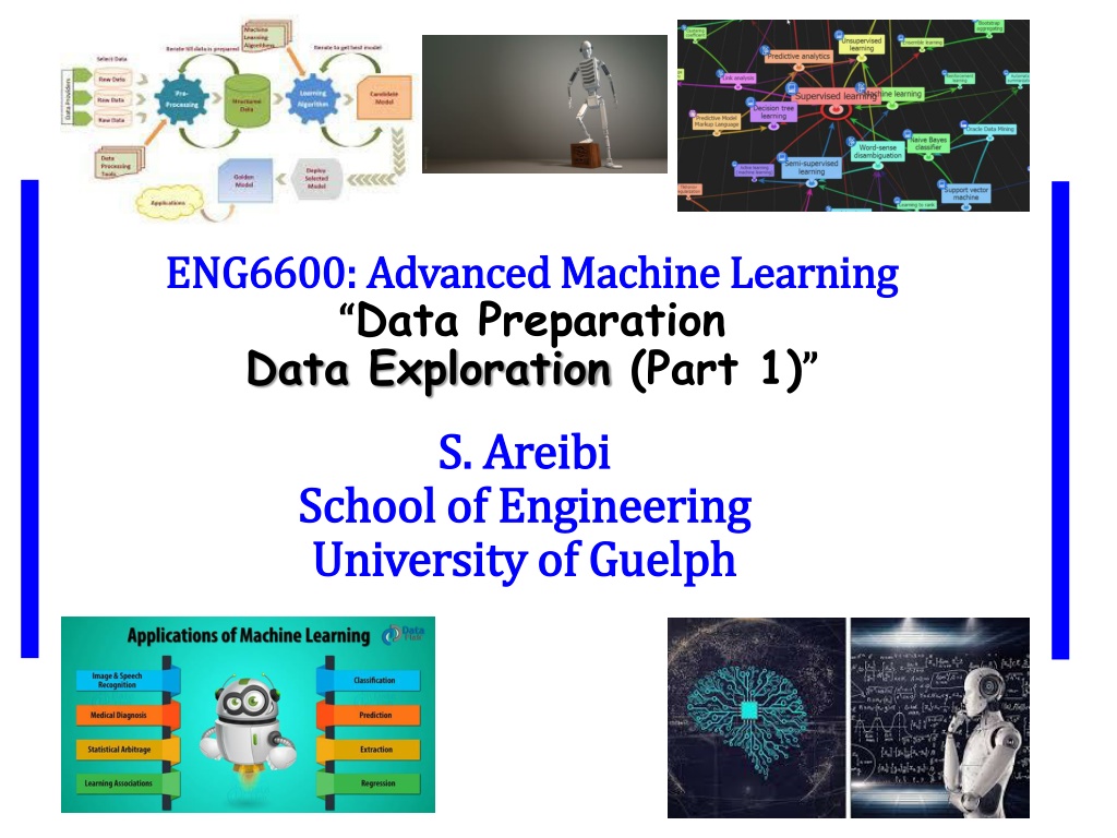


ENG6600: Advanced Machine Learning
“
Data Preparation
Data Exploration
Data Exploration
(Part 1)
”


S. Areibi
School of Engineering
University of Guelph


Week #2
Week #2
Topics Covered
Topics Covered
ML: Data Preparation
ML: Data Preparation
•
This week we will cover and learn the following topics:
1.
The
ML Process
in more detail
2.
Data Understanding
3.
Data Sources
4.
Types of Data
5.
Data Exploration
6.
Data Preparation
•
(a) Selection, (b) Preprocessing, (c) Transformation)
7.
Data Scaling
•
(a) Normalization, (b) Standardization
8.
Feature Selection
and Reduction
9.
Data Balancing
:
•
(a) Resampling, (b) Adjusting Class Weights
3
ML Process and Steps
ML Process and Steps
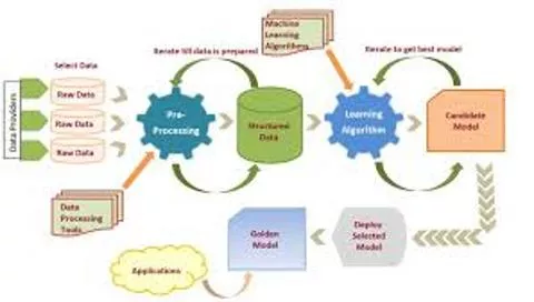
Applied ML Process
Applied ML Process
o
The
process
process
of applied machine learning consists of a
sequence of steps
sequence of steps
.
o
The
steps
steps
are the same
are the same
, but the names of the steps and
tasks performed may differ
tasks performed may differ
from description to description.
o
Here are the
four high-level steps
four high-level steps
:
Step 1
:
Define Problem
Define Problem
o
(
Understand
…Regression/Classification .. Clustering .. Explore Data)
Step 2
:
Prepare Data
Prepare Data
o
(
Clean data
, Preprocess data, Transform data …)
Step 3
:
Select and Evaluate Models
Select and Evaluate Models
o
(
Choose appropriate models
, Evaluate, Fine Tune, Revaluate…)
Step 4
:
Finalize Model
Finalize Model
o
(
Deploy model
“Based on evaluation criteria”)
5
Step (1) Define Problem
Step (1) Define Problem
o
This step
This step
is concerned with
learning
enough
about the
project
to select the framing or framings of the prediction task.
a)
Should we use Machine Learning to solve such problem?
b)
Is it
classification
classification
or
regression
regression
, or some other higher-order
problem type?
c)
Should we use
supervised
supervised
or
unsupervised
unsupervised
approaches?
o
It also involves:
a)
Collecting the data
Collecting the data
that is believed to be useful in making a
prediction and defining the form the prediction will take.
b)
It may also involve
talking to project stakeholders
talking to project stakeholders
and other
people with deep expertise in the domain.
o
This step also involves
taking a close look at the data
taking a close look at the data
, as well as
perhaps “
initial
”
data exploration
data exploration
using summary
statistics
and
data
visualization
.
6
Step (2) Prepare Data
Step (2) Prepare Data
o
This step is concerned with
transforming the raw data
transforming the raw data
that
was collected
into a form
into a form
that
can be used
can be used
in modeling.
o
We can define
data preparation
data preparation
as the transformation of raw
data
into a form
into a form
that is
more suitable for modeling
more suitable for modeling
.
o
On a predictive modeling project, such as classification
raw data
raw data
typically
typically
cannot be used directly
(
why
?
)
o
This is because of
reasons such as
:
1)
Requires Data integration,
Combining data from multiple sources
2)
Machine Learning (ML) algorithms
require data to be numeric
.
3)
Some ML algorithms
impose requirements
impose requirements
on the data
(
(
Scaling
…)
4)
Statistical
noise and errors
in the data may
need to be corrected
5)
Data
may not be balanced
favoring one class over another ..
6)
Data my have
outliers
that impede the capability of the ML model
7
(2) Prepare Data .. Cont
(2) Prepare Data .. Cont
o
Data preparation
Data preparation
goes by many names such as ``Data wrangling”,
``Data Cleaning”, ``Data Transformation”, ``Data Preprocessing”,
.. Data preparation can be a painstakingly laborious process.
o
Data Preparation
Data Preparation
(pre-processing)
(pre-processing)
techniques generally refer to the
addition
,
deletion
, or
transformation
of training set data.
o
There are
common or standard tasks
common or standard tasks
that you may use during the
data preparation
data preparation
step in a ML project, including:
1)
More Data Exploration
More Data Exploration
: Relationship between features and label
2)
Data Cleaning
Data Cleaning
: Identifying and
correcting mistakes
and errors in the data.
3)
Feature Selection
Feature Selection
: Identifying the input variables that are
most relevant
to
the task at hand.
4)
Dimensionality Reduction
Dimensionality Reduction
: Create compact projections of the data.
5)
Data Transformation
Data Transformation
: Changing
the scale
or
distribution
of variables
6)
Feature Engineering
Feature Engineering
: Deriving new independent variables from available
data that were missing.
8
Step (3) Select Models
Step (3) Select Models
o
Choose
appropriate
ML models
ML models
for the task in hand.
o
This step is concerned with
properly evaluating
machine learning
machine learning
models
models
on your dataset using metrics (MAE, MSE, RMSE, R
2
, …)
o
This involves tasks such as
selecting a performance metric
selecting a performance metric
for
evaluating the skill of a model,
establishing a baseline
or floor in
performance to which all model evaluations can be compared.
o
It requires that you
design a robust test harness
design a robust test harness
used to evaluate
your models …
avoid overfitting
and
underfitting
o
Examine
factors that may affect the performance
factors that may affect the performance
of the Machine
Learning Algorithm including ..
(a)
Feature Selection
, (b)
, (b)
Data Balancing
o
This step also involves tasks for getting the most out of well-
performing models such as
Hyper Parameter Tuning
(
HPT
)and
deploying
ensemble based models
or more traditional models.
9
Step (4) Finalize Model
Step (4) Finalize Model
o
This step is concerned with
selecting, and
deploying
a final model.
o
Once
a suite of models has been evaluated
, you must
choose a
choose a
model
model
that represents the “solution” to the project. This is called
model selection
and may involve further evaluation of candidate
models on a hold out validation dataset, or selection via other project-
specific
criteria
criteria
such as
cost
, maintenance, portability ..
o
It may also involve
summarizing the performance of the model
summarizing the performance of the model
in a
standard way for project stakeholders, which is an important step.
o
Finally, there will likely be
tasks related to the deployment
tasks related to the deployment
of the
model, such as:
o
Integration into a
software project.
??
o
Integration into a
CAD flow
??
o
Integration into a
hardware project
. ??
10
What are the most important factors beside accuracy/performance?
•
Ease of Deployment
•
Simplicity of HPT
•
Inference
Time
11
Designing an ML Solution
Designing an ML Solution
Real Data vs. Synthetic Data … Advantages/Disadvantages??
Source of data?
Data Ingredients
Reading/compiling Data?
•
More Flexible
•
Test what if scenarios
•
Test a hypothesis
•
Represent any situation
•
….
Data
Data
Data Understanding: Quantity
Data Understanding: Quantity
Number of instances
(Records?) …
Enough for training?
•
Rule of thumb:
500
-
5,000 desired
•
If less, results are less reliable; use special methods (boosting, …)
Number of attributes
(Fields?) …
Meaningful Features?
•
Rule of thumb: for each field,
10 or more instances
•
If more fields, use feature reduction and selection
Statistics of attributes
and relationship between features
•
Min, Max, Mean, std deviation, missing values …
Number of targets
(Classes?) ….
Balanced Data?
•
Rule of thumb: >100 for each class
•
if very
unbalanced
, use stratified sampling
13
What are the different types of data
?
14
Data Types
Data Types
1.
Numerical data
Numerical data
, or
quantitative data
, is any form of measurable data such as your
height, weight, or the cost of your phone bill. You can determine if a set of data is
numerical by attempting to average out the numbers or sort them.
2.
Categorical data
Categorical data
is sorted by defining characteristics. This can include gender, social
class, ethnicity, hometown, the industry you work in, or a variety of other labels.
Categorical data is great for
grouping individuals or ideas that share similar attributes
,
helping your machine learning model streamline its data analysis.
3.
Time series data
Time series data
consists of data
points that are indexed at specific points
in time.
The distinct difference between time series data and numerical data is that time
series data has established starting and ending points, while numerical data is simply
a collection of numbers that aren’t rooted in particular time periods.
4.
Text data
Text data
is
simply words
, sentences, or paragraphs that can provide some level of
insight to your machine learning models. Since these words can be difficult for models
to interpret on their own, they are most often grouped together or analyzed using
various methods such as word frequency, text classification, or sentiment analysis.
15
Attributes (Features)
Attributes (Features)
Attribute
(
or
dimensions,
features
, variables
): a data
field, representing a
characteristic/feature
of a data object.
E.g., customer _ID, name, address, weight, …
Types:
Numerical …
Integer .. Floating point .. Fractional
Integer .. Floating point .. Fractional
Nominal:
categories
, states, or “names of things”
Hair_color =
{auburn, black, blond, brown, grey, red, white
}
marital status, occupation, ID numbers, zip codes, gender
Ordinal
Values have a
meaningful order
meaningful order
(ranking) but magnitude between
successive values is not known.
Size =
{small, medium, large
}
,
grades, army rankings
Binary
Nominal attribute with only
2 states
(0 and 1)
Symmetric binary
: both outcomes equally important
o
e.g.,
gender, Pass/No Pass, Sick/Healthy
Asymmetric binary
: outcomes not equally important.
e.g.,
medical test (positive vs. negative)
16
Categorical Data
Categorical Data
Categorical data
Categorical data
is data that takes only a limited number of values
One-Hot Encoding
is used in machine learning as a
method to quantify
categorical data
.
In short, this method
produces a vector
produces a vector
with length equal to the number of
categories in the data set. If a data point belongs to the i
th
category then
components of this vector are assigned the value 0 except for the ith component,
which is assigned a value of 1. In this way one can keep track of the categories in a
numerically meaningful way.
One hot encoding
creates new (binary) columns,
indicating the presence of each
possible value from the original data
.
One hot encoding
is the
most widespread approach
, and
it works very well
unless
your categorical variable takes on a large number of values (i.e. you generally won't
it for variables taking more than 15 different values. It'd be a poor choice in some
cases with fewer values, though that varies.)
Not all ML models can
accept
categorical
data and therefore a
method is required to
quantify these values
17
Structured vs Unstructured
Structured vs Unstructured
Data comes in two formats (
structured
,
Unstructured
)
Structured
vs.
unstructured
data
can be understood
can be understood
by
considering the
who
,
what
,
when
,
where
, and the
how
of the
data:
1.
Who
created the data?
2.
Who
will be using the data?
3.
What
type of data are you collecting?
4.
When
does the data need to be prepared, before storage
or when used?
5.
Where
will the data be stored?
6.
How
will the data be stored?
18
Structured Data
Structured Data
Structured data
Structured data
is data that
has been predefined
and
formatted to a set structure
before being placed in data
storage (predefined format)
The best example of
structured data
structured data
is the
relational
database
: the data has been formatted into
precisely
defined fields
such as name, address, .. In order to be
easily queried with SQL ..
Pros of
structured data
structured data
:
1.
Easily used
by machine learning algorithms
2.
Easily used
by business users
3.
Increases access to more tools.
Cons of
structured data
structured data
: (
lack of flexibility
)
1.
A predefined purpose limits use (
limited flexibility
limited flexibility
)
2.
Limited storage
Limited storage
options
19
Unstructured Data
Unstructured Data
Unstructured data
Unstructured data
is data
stored in its
native format
and
not processed until it is used.
Unstructured data
Unstructured data
comes in a myriad of file formats,
including
email, social media posts, presentations, chats,
IoT sensor data, and satellite imagery, audio, images ..
.
Pros of
Unstructured Data
Unstructured Data
:
1.
Freedom of the native format
2.
Faster Accumulation Rate
3.
Data Lake Storage
Easily stored anywhere
.
Cons of
Unstructured Data
Unstructured Data
1.
Requires
Requires
data science
expertise to prepare and analyze
it.
2.
Requires
Requires
specialized tools to manipulate
.
Data
Data
Sources
Sources
ML Data Sources
ML Data Sources
21
There are many sites that offer free data including
ML Data Sources
ML Data Sources
22
Google’s Dataset Search
Google’s Dataset Search
:
Google released their
Google Dataset Search Engine
in
September 2018. This is a popular ML dataset resource that
can help you find
unique
machine learning data
…. https://datasetsearch.research.google.com/
Microsoft Research Open Data
Microsoft Research Open Data
:
Microsoft is another technological leader who has created
a database of free, curated datasets in the form of
Microsoft Research Open Data
. These
datasets are available to the public and are used to “advance state-of-the-art research in
areas such as
natural language processing
,
computer vision
,, and domain specific
sciences.”
….
https://www.microsoft.com/en-us/research/project/microsoft-research-open-data/
Amazon Datasets
Amazon Datasets
:
Amazon Web Services (AWS) has grown to be one of the largest on-
demand cloud computing platforms in the world. With so much data being stored on
Amazon’s servers, a plethora of datasets have been made available to the public through
AWS resources.
Amazon Datasets include,
Commerce Reviews, Transportation,
economy, health and education.
•
UCI Machine Learning Repository
UCI Machine Learning Repository
:
The University of California, provides a large amount
of information to the public through its
UCI Machine Learning Repository
database. This
database is prime for machine learning data as it includes nearly
500 datasets
, (
some of
the most popular datasets used in ML are from UCI
) domain theories, and data
generators which are used for “the empirical analysis of machine learning algorithms.”
•
Government Datasets
Government Datasets
:
The United States Government has released several datasets for
public use. As another great avenue for machine learning data, these datasets can be
used for
conducting research, creating data visualizations, developing web/mobile
applications, and more. The US Government database can be found at
Data.gov
23
ML Data Sources
ML Data Sources
SKLearn:
SKLearn:
Loading
Loading
Data
Data
Load ML Data in Python
Load ML Data in Python
Developers should be able to
load their data
load their data
before they can start
their machine learning project.
Input data sets can be in
various formats
:
(
.XLS, .TXT, .CSV, JSON
).
In Python, it is easy to load data from any source, due to its simple
syntax and availability of
predefined libraries, such as Pandas.
predefined libraries, such as Pandas.
Pandas are used extensively to open and load datasets.
Pandas features
a number of functions
for reading tabular data
as a
Pandas DataFrame
object.
Below are the
common functions
that can be used to read data
(including read_csv in Pandas):
25
Load ML Data in Python
Load ML Data in Python
The
most common format
most common format
for machine learning data is
CSV files
.
There are a number of ways to load a CSV file in Python.
There are a number of considerations when loading your machine
learning data from
CSV files
:
o
CSV File Header
CSV File Header
: If a header is
included
this would
help identify a name
for each attribute
. If not, then you will need to name attributes manually.
o
Comments
Comments
: All
comments
comments
are indicated by a
hash (#).
If you have comments
in your file, depending on the method used to load your data, you may need
to indicate whether or not to expect comments.
o
Delimiter
Delimiter
: The
standard delimiter
that separates values in fields is the
comma (“,”)
character. Some files could use a different delimiter like tab in
which case you must specify it explicitly.
o
Quotes
Quotes
: Sometimes field values can have spaces. In these CSV files the
values are often quoted. The default quote character is “\””
26
Load CSV with Python SL
Load CSV with Python SL
o
The Python API provides the module
CSV
and the function
csv.reader
()
()
that can be used to load
CSV
files.
o
Once loaded, you convert the
CSV
data to a
NumPy array
and use
it for machine learning.
27
# Load CSV (using python)
import csv
import numpy
filename
= 'pima-indians-diabetes.data.csv'
raw_data =
open
(
filename
, 'rt')
reader =
csv.reader
(raw_data, delimiter=',', quoting=csv.QUOTE_NONE)
x = list(reader)
data
= numpy.array(x).astype('float')print(
data.shape
)
The example loads an object that can iterate over each row of the data and can easily be
converted into a NumPy array. Running the example prints the shape of the array.
(768, 9)
Load CSV with NumPy
Load CSV with NumPy
o
You can load your
CSV
data
using NumPy
and the
numpy.loadtxt
() function.
o
This function
assumes no header row
assumes no header row
and all data has the same
format.
o
The example below assumes that the file
pima-indians-
diabetes.data.csv
is in your current working directory.
28
# Load CSV using
NumPy
import numpy
filename
= 'pima-indians-diabetes.data.csv'
raw_data = open(
filename
, 'rt’)
data =
numpy.loadtxt
(raw_data, delimiter=",")
print(data.shape)
Running the example prints the shape of the array.
(768, 9)
Load CSV with NumPy
Load CSV with NumPy
o
The same example can be modified slightly to load the same dataset
directly
from a URL
(
urlopen
)
as follows:
29
# Load CSV from URL using
NumPy
from numpy import loadtxt
from urllib.request import urlopen
url = 'https://raw.githubusercontent.com/jbrownlee/Datasets/master/pima-indians-diabetes.data.csv'
raw_data
=
urlopen
(
url
)
dataset = loadtxt(
raw_data
, delimiter=",")
print(dataset.shape)
Running the example prints the shape of the array.
(768, 9)
Load CSV with Pandas
Load CSV with Pandas
o
You can load your CSV data
using Pandas
and the function
pandas.read_csv
() .
o
This function is very flexible and is perhaps the
recommended
recommended
approach
approach
for loading your machine learning data.
o
The function
returns a pandas.DataFrame
that you can
immediately start summarizing and plotting.
30
Running the example prints the shape of the array.
(768, 9)
# Load CSV using
Pandas
import pandas
filename
= 'pima-indians-diabetes.data.csv'
names = ['preg', 'plas', 'pres', 'skin', 'test', 'mass', 'pedi', 'age', 'class']
data =
pandas.read_csv
(
filename
, names=names)
print(data.shape)
Load CSV with Pandas
Load CSV with Pandas
o
You can load your CSV data using Pandas and the function
pandas.read_csv
() from
a URL
a URL
.
31
Running the example prints the shape of the array.
(768, 9)
# Load CSV
using Pandas
from URL
import pandas
url
= "https://raw.githubusercontent.com/jbrownlee/Datasets/master/pima-indians-diabetes.data.csv"
names = ['preg', 'plas', 'pres', 'skin', 'test', 'mass', 'pedi', 'age', 'class']
data =
pandas.read_csv
(
url
, names=names)
print (data.shape)
Load CSV with Pandas
Load CSV with Pandas
o
Use
data.info
()
32
Running the example prints
the features (columns)
and
Data Type of each feature
.
# Load CSV using
Pandas from URL
import pandas
url
= "https://raw.githubusercontent.com/jbrownlee/Datasets/master/pima-indians-diabetes.data.csv"
names = ['preg', 'plas', 'pres', 'skin', 'test', 'mass', 'pedi', 'age', 'class']
data =
pandas.read_csv
(
url
, names=names)
data.info()
<class 'pandas.core.frame.DataFrame'>
RangeIndex: 768 entries, 0 to 767
Data columns (total 9 columns):
# Column Non-Null Count Dtype
--- ------ -------------- -----
0 preg 768 non-null int64
1 plas 768 non-null int64
2 pres 768 non-null int64
3 skin 768 non-null int64
4 test 768 non-null int64
5 mass 768 non-null float64
6 pedi 768 non-null float64
7 age 768 non-null int64
8 class 768 non-null int64
dtypes: float64(2), int64(7)
memory usage: 54.1 KB
Load CSV with Pandas
Load CSV with Pandas
o
Use
data.describe
()
33
Running the example prints the
features (columns) and Stats
# Load CSV using Pandas from URL
import pandas
url
= "https://raw.githubusercontent.com/jbrownlee/Datasets/master/pima-indians-diabetes.data.csv"
names = ['preg', 'plas', 'pres', 'skin', 'test', 'mass', 'pedi', 'age', 'class']
data =
pandas.read_csv
(
url
, names=names)
data.describe()
preg
plas
pres
skin
test
mass
pedi
age
class
count
768.000000
768.000000
768.000000
768.000000
768.000000
768.000000
768.000000
768.000000
768.0000
mean
3.845052
120.894531
69.105469
20.536458
79.799479
31.992578
0.471876
33.240885
0.348958
std
3.369578
31.972618
19.355807
15.952218
115.244002
7.884160
0.331329
11.760232
0.476951
min
0.000000
0.000000
0.000000
0.000000
0.000000
0.000000
0.078000
21.000000
0.000000
25%
1.000000
99.000000
62.000000
0.000000
0.000000
27.300000
0.243750
24.000000
0.000000
50%
3.000000
117.000000
72.000000
23.000000
30.500000
32.000000
0.372500
29.000000
0.000000
75%
6.000000
140.250000
80.000000
32.000000
127.250000
36.600000
0.626250
41.000000
1.000000
max
17.000000
199.000000
122.000000
99.000000
846.000000
67.100000
2.420000
81.000000
1.000000
SKLearn:
SKLearn:
Synthetic
Synthetic
Data
Data
Synthetic Data
Synthetic Data
The performance of machine learning algorithms such as
classification, clustering, regression, decision trees or neural
networks
can be significantly improved
with
synthetic data
.
It
enriches training sets
, allowing you to make predictions or
assign a label to new observations that are significantly different
from those in your dataset.
It is very useful
if your training set
is
small
or
unbalanced
.
It also allows you to
test the limits of your algorithms
and
find examples where it fails to work
(for instance, failing to
identify spam). Or deal with missing data or create confidence
regions for parameters.
Data Scientists should learn different techniques on how to design
rich,
good quality synthetic data
to meet all these goals.
35
Creating Synthetic Data
Creating Synthetic Data
Synthetic data can be
very useful
for the following reasons:
You can
generate
as much synthetic data
as much synthetic data
as you need,
You can generate data that may be
dangerous to collect
dangerous to collect
in reality,
Synthetic data is
automatically annotated
.
Among their many advantages,
synthetic datasets
synthetic datasets
are
free from
personal data
and therefore not subject to compliance restrictions
or other privacy protection laws,
SKLearn
SKLearn
allows users to create synthetic data
which might be
useful if you
lack datasets
or if you wish to
create data with
specific features
.
Data can be created for either
regression or classification
regression or classification
.
An example of creating and summarizing the synthetic data set is
given next.
36
https://machinelearningmastery.com/clustering-algorithms-with-python/
Creating Synthetic Data
Creating Synthetic Data
37
# synthetic classification dataset
from numpy import
where
from sklearn.datasets import
make_classification
from matplotlib import
pyplot
# define dataset
X, y =
make_classification
(n_samples=1000, n_features=2, n_informative=2, n_redundant=0,
n_clusters_per_class=1, random_state=4)
# create scatter plot for samples from each class
for class_value in range(2):
# get row indexes for samples with this class
row_ix =
where
(y == class_value)
# create scatter of these samples
pyplot.scatter(X[row_ix, 0], X[row_ix, 1])
# show the plot
pyplot
.show()
The
make_classification
function can be
called from sklearn library with the following
options:
1)
Number of samples n_samples
2)
Number of features n_features
3)
Number of informative features
Data
Data
Exploration
Exploration
Data Exploration
Data Exploration
o
Data Exploration
refers to the
initial step in data analysis
initial step in data analysis
in which data
analysts use
data visualization
and
statistical techniques
to
describe
dataset characterizations
, such as
size
,
quantity
,
feature relationship
and
accuracy, in order to better understand the nature of the data.
o
Starting with
Starting with
data exploration
data exploration
helps users to
make better decisions
on
where to dig deeper into the data and to take a broad understanding of the
business when asking more detailed questions later.
o
Data exploration is easy with Python and Scikit Learn
Data exploration is easy with Python and Scikit Learn
o
Data exploration
Data exploration
with python
has the advantage in
ease of learning
ease of learning
,
production readiness, integration with common tools, an
abundant library
, and
support from a huge community.
o
Python data exploration
Python data exploration
is
made easier with Pandas
made easier with Pandas
, the open source
Python data analysis library that can single-handedly profile any dataframe and
generate a complete HTML report on the dataset.
o
Once Pandas is imported, it allows users to import files in a variety of formats,
the most
popular format being CSV
popular format being CSV
.
39
Data Exploration
Data Exploration
Here are
some of the tasks
some of the tasks
and operations we will cover after loading a
datafile using Pandas:
1.
How to print
How to print
the
first few
and last few
records
in a dataset.?
2.
Identifying
Identifying
the number of
rows
(records) and
columns
(features)
3.
How to print
How to print
statistics
of
features
within the dataset? Min, max, ..
4.
How to identify
How to identify
rows that contain
missing values
?
5.
How to plot
How to plot
the
distribution of classes
in a dataset?
6.
How to plot
How to plot
the
Correlation Matrix
that represents the
`correlation’ between pairs of variables in a given data?
7.
Introduce
Introduce
the
correlation coefficient
which is the number that
denotes the strength of the relationship between two variables.
8.
How to create plots
How to create plots
(Histogram, Scatter, Box Plot)?
9.
How to generate
How to generate
frequency tables?
40
Correlation Matrix
Correlation Matrix
Correlation Matrix
Correlation Matrix
o
A
Correlation Matr
Correlation Matr
ix
ix
is a tabular data representing the `correlation’
between pairs of variables in a given data
o
The matrix below shows the
Correlation Matrix
Correlation Matrix
of Breast Cancer Data.
o
Each row and column represents a variable (feature), and
each value in
each value in
this matrix
this matrix
is the
Correlation Coefficient
Correlation Coefficient
between the variables
represented by the corresponding row and column.
42
Very Low Correlation
Very Low Correlation
Correlation Matrix
Correlation Matrix
o
The
Correlation Matrix
Correlation Matrix
is an
important data analysis metric
important data analysis metric
that is
computed to summarize data to
understand the relationship
understand the relationship
between various variables
between various variables
and make decisions accordingly.
o
It is also an
important pre-processing step
important pre-processing step
in Machine Learning
pipelines to compute and analyze the
Correlation Matrix
Correlation Matrix
where
dimensionality reduction is desired
dimensionality reduction is desired
on a high-dimension data.
o
Each cell
in
Correlation Matrix
Correlation Matrix
is a ‘
correlation coefficient
correlation coefficient
‘
between the two variables corresponding to the row and column of the
cell.
43
What is the correlation coefficient?
Correlation Coefficient
Correlation Coefficient
o
A
correlation coefficient
correlation coefficient
is a number that
denotes the
strength
strength
of
the relationship
between two variables.
o
There are
several types of
correlation coefficients
correlation coefficients
, but the
most common
of them all is the
Pearson’s coefficient
Pearson’s coefficient
denoted by
the Greek letter ρ (rho). Others:
Spearmans coefficient
Kendal Tau correlation coefficient
o
It is
defined as
defined as
the
covariance between two variables
divided
by the
product of
the
standard deviations
of the two variables.
44
Correlation Coefficient
Correlation Coefficient
o
Where the covariance between X and Y
COV(X,Y)
COV(X,Y)
is further defined as
the `
expected value
expected value
of the
product of
the
deviation of X and Y
from
their respective means’.
o
The formula for covariance would make it clearer:
45
o
So, the formula for
Pearson’s correlation
would then become:
o
The value of rho lies between +1 and -1.
o
Values nearing
+1
+1
indicate the presence of a
strong positive relation
strong positive relation
between X and Y, whereas those nearing
-1
indicate a
strong negative
relation between X and Y
.
o
Values near to zero
Values near to zero
mean there is an
absence of any relationship.
Python Code:
Python Code:
Two Vars
Two Vars
•
The code below generates random data for two variables and then constructs the
correlation matrix
46
import numpy as np
np.random.seed(10)
# generating 10 random values for each of the two variables
X = np.random.randn(10)
Y = np.random.randn(10)
# computing the correlation matrix
C = np.corrcoef(X,Y)
print(C)
[[ 1.0 0.0247439
[0.0247439 1.0
•
The
value 0.02
indicates there
doesn’t exist a relationship between the two
variables
. This was expected since their values were generated randomly.
•
In this example, we used NumPy’s `corrcoef` method to generate the correlation
matrix.
•
However,
this method has a limitation
this method has a limitation
in that it can compute the correlation matrix
between
2 variables only
.
Python Code:
Python Code:
Multiple Vars
Multiple Vars
•
The code below constructs the correlation matrix for multiple variables
•
We will use the Breast Cancer data.
47
from sklearn.datasets import load_breast_cancer
import pandas as pd
breast_cancer =
load_breast_cancer()
data = breast_cancer.data
features = breast_cancer.feature_names
df = pd.DataFrame(data, columns = features)
print(
df.shape
)
print(features)
Python Code: Multiple Vars
Python Code: Multiple Vars
•
We will plot the relationship between each pair of the features.
•
However, to keep things simple, we will use the
first 6 features
first 6 features
and plot.
48
import seaborn as sns
import matplotlib.pyplot as plt
# taking all rows but only 6 columns
df_small = df.iloc[:,:6]
correlation_mat
=
df_small.
corr()
sns.heatmap(
correlation_mat
, annot = True)
plt.show()
•
Pandas DataFrame’s
corr()
method
is used to compute the matrix. By
default, it computes the Pearson’s
correlation coefficient
.
•
We
could also use other methods
could also use other methods
such as
Spearman’s coefficient
or
Kendall Tau
correlation coefficient
by passing an appropriate value to
the parameter 'method'.
Python Code: Multiple Vars
Python Code: Multiple Vars
•
Each cell
Each cell
in the grid represents the value of the correlation coefficient between two variables.
•
The
value at position (a, b)
represents the correlation coefficient between features at row a and
column b. This will be equal to the value at position (b, a)
•
It is a
square matrix
square matrix
– each row represents a variable, and all the columns represent the same
variables as rows, hence the number of rows = number of columns.
•
It is a
symmetric matrix
symmetric matrix
– this makes sense because the correlation between a,b will be the same as
that between b, a.
•
All diagonal elements are 1
All diagonal elements are 1
. Since diagonal elements represent the correlation of each variable with
itself, it will always be equal to 1.
•
The axes ticks denote the feature each of them represents.
49
Python Code: Multiple Vars
Python Code: Multiple Vars
•
A
large positive value
(near to 1.0) indicates a
strong positive correlation
, i.e., if the value of one of
the variables increases, the value of the other variable increases as well.
•
A
large negative value
(near to -1.0) indicates a
strong negative correlation
, i.e., the value of one
variable decreases with the other’s increasing and vice-versa.
•
A value near to 0
(both positive or negative) indicates the
absence of any correlation
between the
two variables, and hence those
variables are independent
of each other.
•
Each cell in the above matrix is also represented by shades of a color. Here darker shades of the
color indicate smaller values while brighter shades correspond to larger values (near to 1).
•
This scale is given with the help of a color-bar on the right side of the plot.
50
Correlation Coefficient
Correlation Coefficient
51
Observations:
•
To fit a linear regression model, we
select those features which have a high
correlation with
our target variable
MEDV.
•
By looking at the correlation matrix we can see that RM has a strong positive
correlation with MEDV (0.7) where as LSTAT has a high negative correlation with
MEDV(-0.74).
Correlation Coefficient
Correlation Coefficient
52
Observations:
•
An important point in selecting features for a linear regression model is to
check
for multi-co-linearity
.
•
The features
RAD, TAX have a
correlation of 0.91
.
•
These feature pairs are
strongly correlated to each other
.
•
We should not select both
these features
together for training the model.
•
Same goes for the features DIS and AGE which have a correlation of -0.75.
SK-Learn: Data Exploration
SK-Learn: Data Exploration
Iris: Data Exploration
Iris: Data Exploration
o
The dataset to be used is called ``iris flowers” which is a standard
machine learning dataset.
o
Information about this dataset can be found at the following link:
https://raw.githubusercontent.com/jbrownlee/Datasets/master/iris.names
o
The dataset involves
predicting the flower species
predicting the flower species
given
measurements of iris flowers in centimeters.
o
It is a
multi-class classification problem
multi-class classification problem
. The number of
observations for each class is balanced.
o
There are
150 observations
150 observations
with
4 input variables
and
1 output
variable
.
54
Iris: Data Exploration
Iris: Data Exploration
o
The iris dataset can be accessed from the following link
https://raw.githubusercontent.com/jbrownlee/Datasets/master/iris.csv
o
The first few lines of the file should look as follows:
55
5.1,3.5,1.4,0.2,Iris-setosa
4.9,3.0,1.4,0.2,Iris-setosa
4.7,3.2,1.3,0.2,Iris-setosa
4.6,3.1,1.5,0.2,Iris-setosa
5.0,3.6,1.4,0.2,Iris-setosa
o
The
4
4
attributes
attributes
are, (a) Sepal Length, (b) Sepal Width, (c) Petal
Length, (d) Petal Width ..
o
There are
3 classes
3 classes
(a) Setosa, (b) Versicolour, (c) Virginica
o
Class Distribution: 33.3% for each of the 3 classes.
Iris: Data Exploration
Iris: Data Exploration
56
# Exploring Iris Dataset
# Import necessary libraries
import pandas as pd
import numpy as np
import matplotlib.pyplot as plt
import seaborn as sns
from scipy.stats import norm
from scipy import stats
from pandas import read_csv
Iris: Data Exploration
Iris: Data Exploration
57
# define the location of the dataset
# path = 'https://raw.githubusercontent.com/jbrownlee/Datasets/master/iris.csv'
path = 'iris_mod.csv'
# load the dataset and use df as a data frame
iris_df =
read_csv
(path, header=None)
# show the first few rows of the data
iris_df.
head
()
0
1
2
3
4
0
5.1
3.5
1.4
0.2
0
1
4.9
3.0
1.4
0.2
0
2
4.7
3.2
1.3
0.2
0
3
4.6
3.1
1.5
0.2
0
4
5.0
3.6
1.4
0.2
0
5
…… ….. ….. ….. …
6
…… ….. ….. ….. …
Records
Features
Iris: Data Exploration
Iris: Data Exploration
58
# show the names of the columns or features
iris_df.
columns
Int64Index([0, 1, 2, 3, 4], dtype='int64')
# show the number of rows and columns
iris_df.
shape
(150, 5)
# get various summary stats of the data
iris_df.
describe
()
0
1
2
3
4
count
150.000000
150.000000
150.000000
150.000000
150.000000
mean
5.843333
3.054000
3.758667
1.198667
1.000000
std
0.828066
0.433594
1.764420
0.763161
0.819232
min
4.300000
2.000000
1.000000
0.100000
0.000000
25%
5.100000
2.800000
1.600000
0.300000
0.000000
50%
5.800000
3.000000
4.350000
1.300000
1.000000
75%
6.400000
3.300000
5.100000
1.800000
2.000000
max
7.900000
4.400000
6.900000
2.500000
2.000000
Iris: Data Exploration
Iris: Data Exploration
59
# Give some stats of the feature ‘Sepal_length’
iris_df[
'Sepal_length
'].
describe
()
count 150.000000
mean 5.843333
std 0.828066
min 4.300000
25% 5.100000
50% 5.800000
75% 6.400000
max 7.900000
Name: Sepal_length, dtype: float64
Iris: Data Exploration
Iris: Data Exploration
60
# Identify rows that contain missing values
iris_df.
isnull
()
0
1
2
3
4
0
False
False
False
False
False
1
False
False
False
False
False
2
False
False
False
False
False
3
False
False
False
False
False
4
False
False
False
False
False
...
...
...
...
...
...
145
False
False
False
False
False
146
False
False
False
False
False
147
False
False
False
False
False
148
False
False
False
False
False
149
False
False
False
False
False
150 rows × 5 columns
Iris: Data Exploration
Iris: Data Exploration
61
# Assign Names to the Features
names = ['Sepal_length', 'Sepal_width', 'Petal_length', 'Petal_width','Species']
iris_df = read_csv(path, names=names, header=None)
# Show the first few rows of the data again
iris_df.
head
()
Sepal_length Sepal_width Petal_length
Petal_width
Species
0
5.1
3.5
1.4
0.2
0
1
4.9
3.0
1.4
0.2
0
2
4.7
3.2
1.3
0.2
0
3
4.6
3.1
1.5
0.2
0
4
5.0
3.6
1.4
0.2
0
Iris: Data Exploration
Iris: Data Exploration
62
# Seaborn Library
# histogram and Sepal_length Distribution
sns.
displot
(iris_df['Sepal_length'])
Iris: Data Exploration
Iris: Data Exploration
63
# Species Distribution
# Class distribution
sns.
displot
(iris_df[‘Species'])
Scatter Plots
Scatter Plots
64
•
Scatter plots’ primary uses are to
observe and show relationships
observe and show relationships
between two numeric variables
•
Relationships between variables
Relationships between variables
can be described in many ways:
positive or negative, strong or weak, linear or nonlinear.
Scatter Plots
Scatter Plots
65
•
A scatter plot can also be useful for
identifying other patterns in data
.
•
We can divide data points into groups based on how closely sets of
points cluster together
.
•
Scatter plots can also show if there are any
unexpected gaps
in the data
and if there are any
outlier points
.
•
This can be useful if we want to segment the data into different parts,
like in the development of user personas.
Iris: Data Exploration
Iris: Data Exploration
66
%matplotlib inline
import seaborn as sns; sns.set()
sns.pairplot(iris_df, hue='Species', height=1.5);
Iris: Data Exploration
Iris: Data Exploration
67
# Missing Data
# If more than 15% of the data is missing then we might want to
delete the feature
delete the feature
(variable)
total = iris_df.isnull().sum().sort_values(ascending=False)
percent = (iris_df.isnull().sum()/iris_df.isnull().count()).sort_values(ascending=False)
missing_data = pd.concat([total, percent], axis=1, keys=['Total', 'Percent'])
missing_data.head(20)
Total
Percent
Sepal_length
0
0.0
Sepal_width
0
0.0
Petal_length
0
0.0
Petal_width
0
0.0
Species
0
0.0
# Dealing with Missing Data
iris_df = iris_df.drop((missing_data[missing_data['Total'] > 1]).index,1)
## Remove the row where the feature was missing instead of removing the feature column
## iris_df = iris_df.drop(iris_df.loc[df_train['THE-FEATHRE'].isnull()].index)
iris_df.isnull().sum().max() #just checking that there's no missing data missing...
0
Iris: Data Exploration
Iris: Data Exploration
68
# We can extract the feature matrix and target array from the iris
data_frame
#
This would be useful later on when we use Scikit-Learn to perform classification
X_iris = iris_df.drop(‘Species', axis=1)
X_iris.shape
(150, 4)
# We can extract the feature matrix and target array from the iris
data_frame
#
This would be useful later on when we use Scikit-Learn to perform classification
y_iris = iris['species']
y_iris.shape
(150,)
The expected layout of features and target
values is visualized in the following diagram:
Summary
Summary
Summary
Summary
o
Each
machine learning project is different
machine learning project is different
since the specific data at
the core of the project is different.
o
Data Preparation
Data Preparation
may be one of the most
difficult steps
difficult steps
in any
machine learning project.
o
Data preparation
Data preparation
is concerned with
transforming the raw data
transforming the raw data
that
was collected into a form that
can be used in modeling
can be used in modeling
.
o
Data pre-processing techniques generally refer to the
addition,
addition,
deletion
deletion
, or transformation of training set data.
o
Data Exploration
Data Exploration
is one of the steps in data preparation. It is an
approach similar to initial
data analysis
data analysis
, whereby a data analyst
uses
visual exploration
visual exploration
to understand
what is in a dataset
and the
characteristics of the data
, rather than through traditional data
management systems
70
Resources
Resources
Misc. Resources: Data
Misc. Resources: Data
Kaggle:
Kaggle:
https://www.kaggle.com/datasets
https://www.kaggle.com/datasets
UCI:
UCI:
•
http://archive.ics.uci.edu/ml/index.php
http://archive.ics.uci.edu/ml/index.php
•
https://archive.ics.uci.edu/ml/datasets.php
https://archive.ics.uci.edu/ml/datasets.php
KDD:
KDD:
http://kdd.ics.uci.edu/summary.data.application.html
http://kdd.ics.uci.edu/summary.data.application.html
Wikipedia:
Wikipedia:
•
https://en.wikipedia.org/wiki/List_of_datasets_for_machine-learning_research
https://en.wikipedia.org/wiki/List_of_datasets_for_machine-learning_research
MagicData (Training Datase
MagicData (Training Datase
ts)
ts)
•
https://www.magicdatatech.com/datasets?gclid=Cj0KCQiA8vSOBhCkARIsAGdp6RSi_aSI0L7ag9BI8-
https://www.magicdatatech.com/datasets?gclid=Cj0KCQiA8vSOBhCkARIsAGdp6RSi_aSI0L7ag9BI8-
eYT3jYi4-CZ7jEiQlCg454ayvwU1rhHFwLuhwaAtxAEALw_wcB
eYT3jYi4-CZ7jEiQlCg454ayvwU1rhHFwLuhwaAtxAEALw_wcB
Best free Datasets:
Best free Datasets:
https://www.v7labs.com/blog/best-free-datasets-for-machine-learning
https://www.v7labs.com/blog/best-free-datasets-for-machine-learning
Delve:
Delve:
http://www.cs.utoronto.ca/~delve/
http://www.cs.utoronto.ca/~delve/
Stack Overflow:
Stack Overflow:
https://insights.stackoverflow.com/survey
https://insights.stackoverflow.com/survey
Multi-Label Datasets
Multi-Label Datasets
:
:
•
http://manikvarma.org/downloads/XC/XMLRepository.html
http://manikvarma.org/downloads/XC/XMLRepository.html
72
Misc. Resources: Tutorial
Misc. Resources: Tutorial
o
YouTube (Tutorial on using Jupyter)
YouTube (Tutorial on using Jupyter)
•
https://www.youtube.com/watch?v=HW29067qVWk&t=0s
https://www.youtube.com/watch?v=HW29067qVWk&t=0s
o
YouTube
YouTube
(Python Pandas and installing Jupyter
(Python Pandas and installing Jupyter
)
)
•
Python Pandas (Part 1)
Python Pandas (Part 1)
https://www.youtube.com/watch?v=ZyhVh-qRZPA
•
Python Pandas (Part 2)
Python Pandas (Part 2)
https://www.youtube.com/watch?v=zmdjNSmRXF4
https://www.youtube.com/watch?v=zmdjNSmRXF4
•
Python Pandas (Part 3)
Python Pandas (Part 3)
https://www.youtube.com/watch?v=W9XjRYFkkyw
https://www.youtube.com/watch?v=W9XjRYFkkyw
o
Documents:
Documents:
•
Scatter Plots
Scatter Plots
•
https://chartio.com/learn/charts/what-is-a-scatter-plot/
https://chartio.com/learn/charts/what-is-a-scatter-plot/
•
Reading different formats in Python:
Reading different formats in Python:
•
https://lifewithdata.com/2021/12/10/pandas-read_csv-read-a-csv-file-in-python/
https://lifewithdata.com/2021/12/10/pandas-read_csv-read-a-csv-file-in-python/
•
Structured vs unstructured data
Structured vs unstructured data
•
https://www.talend.com/resources/structured-vs-unstructured-
https://www.talend.com/resources/structured-vs-unstructured-
data/#:~:text=Structured%20data%20is%20highly%20specific,employs%20schema%2Don%2Dread
data/#:~:text=Structured%20data%20is%20highly%20specific,employs%20schema%2Don%2Dread
.
.
73
Misc. Resources: Tutorial
Misc. Resources: Tutorial
o
YouTube (Data Preparation in Machine Learning)
YouTube (Data Preparation in Machine Learning)
•
https://www.youtube.com/watch?v=X6zz9Z2KDtU
•
https://www.youtube.com/watch?v=R8zHAlW4b3I
•
https://www.youtube.com/watch?v=kwK6UpN9Sa8
•
https://www.youtube.com/watch?v=LMKFREH5XdQ
•
https://www.youtube.com/watch?v=c5ASFOYd918
•
https://www.youtube.com/watch?v=NEaUSP4YerM
74
Misc. Resources: Tutorial
Misc. Resources: Tutorial
o
Tutorials (Data Exploration):
Tutorials (Data Exploration):
•
https://likegeeks.com/python-correlation-matrix/
https://likegeeks.com/python-correlation-matrix/
•
https://www.analyticsvidhya.com/blog/2015/04/comprehensive-guide-data-exploration-sas-using-python-numpy-scipy-
https://www.analyticsvidhya.com/blog/2015/04/comprehensive-guide-data-exploration-sas-using-python-numpy-scipy-
matplotlib-pandas/
matplotlib-pandas/
•
https://www.datacamp.com/community/tutorials/exploratory-data-analysis-python
https://www.datacamp.com/community/tutorials/exploratory-data-analysis-python
•
https://www.edureka.co/blog/exploratory-data-analysis-in-python/
https://www.edureka.co/blog/exploratory-data-analysis-in-python/
•
https://www.analyticsvidhya.com/blog/2020/11/a-comprehensive-guide-to-learn-the-data-exploration-in-python/
https://www.analyticsvidhya.com/blog/2020/11/a-comprehensive-guide-to-learn-the-data-exploration-in-python/
•
https://www.youtube.com/watch?v=9qg9__n4X2A
https://www.youtube.com/watch?v=9qg9__n4X2A
•
https://www.analyticsvidhya.com/blog/2016/01/guide-data-exploration/
https://www.analyticsvidhya.com/blog/2016/01/guide-data-exploration/
o
Tutorials (Data Preparation):
Tutorials (Data Preparation):
•
https://machinelearningmastery.com/what-is-data-preparation-in-machine-learning/
https://machinelearningmastery.com/what-is-data-preparation-in-machine-learning/
•
https://machinelearningmastery.com/data-preparation-for-machine-learning-7-day-mini-course/
https://machinelearningmastery.com/data-preparation-for-machine-learning-7-day-mini-course/
•
https://algorithmia.com/blog/the-importance-of-machine-learning-data
https://algorithmia.com/blog/the-importance-of-machine-learning-data
•
https://www.analyticsvidhya.com/blog/2021/06/generate-reports-using-pandas-profiling-deploy-using-streamlit/
https://www.analyticsvidhya.com/blog/2021/06/generate-reports-using-pandas-profiling-deploy-using-streamlit/
•
https://machinelearningmastery.com/basic-data-cleaning-for-machine-learning/
https://machinelearningmastery.com/basic-data-cleaning-for-machine-learning/
75
Basic Statistical Descriptions of Data
Basic Statistical Descriptions of Data
•
Motivation
Motivation
–
To better understand the data: central tendency, variation
and spread
•
Data dispersion characteristics
Data dispersion characteristics
–
median, max, min, quantiles, outliers, variance, etc.
•
Numerical dimensions
Numerical dimensions
correspond to sorted intervals
–
Data dispersion: analyzed with multiple granularities of
precision
–
Boxplot or quantile analysis on sorted intervals
•
Dispersion analysis on computed measures
Dispersion analysis on computed measures
–
Folding measures into numerical dimensions
–
Boxplot or quantile analysis on the transformed cube
77
Measuring the Central Tendency
Measuring the Central Tendency
•
Mean (algebraic measure) (sample vs. population)
Mean (algebraic measure) (sample vs. population)
:
Note:
n
is sample size and
N
is population size.
–
Weighted
arithmetic
mean
mean
:
–
Trimmed mean
Trimmed mean
: chopping extreme values
•
Median
Median
:
–
Middle value
Middle value
if odd number of values, or average of the
middle two values otherwise
–
Estimated by interpolation (for
grouped data
):
•
Mode
Mode
–
Value that occurs
most frequently
most frequently
in the data
–
Unimodal, bimodal, trimodal
–
Empirical formula:
78
Symmetric vs. Skewed Data
Symmetric vs. Skewed Data
•
Median, mean and
mode of symmetric,
positively and
negatively skewed data
79
positively skewed
negatively skewed
symmetric
Measuring the Dispersion of Data
Measuring the Dispersion of Data
•
Quartiles, outliers and boxplots
–
Quartiles
: Q
1
(25
th
percentile), Q
3
(75
th
percentile)
–
Inter-quartile range
: IQR = Q
3
–
Q
1
–
Five number summary
: min, Q
1
, median,
Q
3
, max
–
Boxplot
: ends of the box are the quartiles; median is marked; add whiskers, and
plot outliers individually
–
Outlier
: usually, a value higher/lower than 1.5 x IQR
•
Variance and standard deviation (
sample:
s, population:
σ
)
–
Variance
: (algebraic, scalable computation)
–
Standard deviation
s (or
σ
)
is the square root of variance
s
2 (
or
σ
2)
80
Boxplot Analysis
Boxplot Analysis
•
Five-number summary
of a distribution
–
Minimum, Q1, Median, Q3, Maximum
•
Boxplot
–
Data is represented with a box
–
The ends of the box are at the first and third
quartiles, i.e., the height of the box is IQR
–
The median is marked by a line within the box
–
Whiskers: two lines outside the box extended to
Minimum and Maximum
–
Outliers: points beyond a specified outlier
threshold, plotted individually
81
Topic #2 of the course is on “Data Preparation”
• This topic is divided into several parts ..
• Part 1 will concentrate mainly on “Data Exploration”
• We will start by the defining data, features, and how features relate to each other and label ..
• The outcome of this lecture is being able to explore the data to be used for classification or regression
This lecture on advanced machine learning covers topics such as the ML process in detail, data understanding, sources, types, exploration, preparation, scaling, feature selection, data balancing, and more. The ML process involves steps like defining the problem, preparing data, selecting and evaluating models, and finalizing the model. Each step plays a crucial role in the applied machine learning process. Understanding these steps is essential for successfully implementing machine learning solutions.

Download Presentation

Please find below an Image/Link to download the presentation.
The content on the website is provided AS IS for your information and personal use only. It may not be sold, licensed, or shared on other websites without obtaining consent from the author. Download presentation by click this link. If you encounter any issues during the download, it is possible that the publisher has removed the file from their server.
E N D
Presentation Transcript
ENG6600: Advanced Machine Learning ENG6600: Advanced Machine Learning Data Preparation Data Exploration (Part 1) S. Areibi S. Areibi School of Engineering School of Engineering University of Guelph University of Guelph
Week #2 Topics Covered
ML: Data Preparation This week we will cover and learn the following topics: 1. The ML Process in more detail 2. Data Understanding 3. Data Sources 4. Types of Data 5. Data Exploration 6. Data Preparation (a) Selection, (b) Preprocessing, (c) Transformation) 7. Data Scaling (a) Normalization, (b) Standardization 8. Feature Selection and Reduction 9. Data Balancing: (a) Resampling, (b) Adjusting Class Weights 3
Applied ML Process o The process of applied machine learning consists of a sequence of steps. o The steps are the same, but the names of the steps and tasks performed may differ from description to description. o Here are the four high-level steps: Step 1: Define Problem o (Understand Regression/Classification .. Clustering .. Explore Data) Step 2: Prepare Data o (Clean data, Preprocess data, Transform data ) Step 3: Select and Evaluate Models o (Choose appropriate models, Evaluate, Fine Tune, Revaluate ) Step 4: Finalize Model o (Deploy model Based on evaluation criteria ) 5
Step (1) Define Problem o This step is concerned with learning enough about the project to select the framing or framings of the prediction task. a) Should we use Machine Learning to solve such problem? b) Is it classification or regression, or some other higher-order problem type? c) Should we use supervised or unsupervised approaches? o It also involves: a) Collecting the data that is believed to be useful in making a prediction and defining the form the prediction will take. b) It may also involve talking to project stakeholders and other people with deep expertise in the domain. o This step also involves taking a close look at the data, as well as perhaps initial data exploration using summary statistics and data visualization. 6
Step (2) Prepare Data o This step is concerned with transforming the raw data that was collected into a form that can be used in modeling. o We can define data preparation as the transformation of raw data into a form that is more suitable for modeling. o On a predictive modeling project, such as classification raw data typically cannot be used directly (why?) o This is because ofreasons such as: 1) Requires Data integration, Combining data from multiple sources 2) Machine Learning (ML) algorithms require data to be numeric. 3) Some ML algorithms impose requirements on the data (Scaling ) 4) Statistical noise and errors in the data may need to be corrected 5) Data may not be balanced favoring one class over another .. 6) Data my have outliers that impede the capability of the ML model 7
(2) Prepare Data .. Cont o Data preparation goes by many names such as ``Data wrangling , ``Data Cleaning , ``Data Transformation , ``Data Preprocessing , .. Data preparation can be a painstakingly laborious process. o Data Preparation (pre-processing) techniques generally refer to the addition, deletion, or transformation of training set data. o There are common or standard tasks that you may use during the data preparation step in a ML project, including: 1) More Data Exploration: Relationship between features and label 2) Data Cleaning: Identifying and correcting mistakes and errors in the data. 3) Feature Selection: Identifying the input variables that are most relevant to the task at hand. 4) Dimensionality Reduction: Create compact projections of the data. 5) Data Transformation: Changing the scale or distribution of variables 6) Feature Engineering: Deriving new independent variables from available data that were missing. 8
Step (3) Select Models o Chooseappropriate ML models for the task in hand. o This step is concerned with properly evaluating machine learning models on your dataset using metrics (MAE, MSE, RMSE, R2, ) o This involves tasks such as selecting a performance metric for evaluating the skill of a model, establishing a baseline or floor in performance to which all model evaluations can be compared. o It requires that you design a robust test harness used to evaluate your models avoid overfittingand underfitting o Examine factors that may affect the performance of the Machine Learning Algorithm including .. (a) Feature Selection, (b) Data Balancing o This step also involves tasks for getting the most out of well- performing models such as Hyper Parameter Tuning (HPT)and deploying ensemble based models or more traditional models. 9
Step (4) Finalize Model o This step is concerned with selecting, and deployinga final model. o Once a suite of models has been evaluated, you must choose a model that represents the solution to the project. This is called model selection and may involve further evaluation of candidate models on a hold out validation dataset, or selection via other project- specific criteria such as cost, maintenance, portability .. o It may also involve summarizing the performance of the model in a standard way for project stakeholders, which is an important step. o Finally, there will likely be tasks related to the deployment of the model, such as: o Integration into a software project. ?? o Integration into a CAD flow ?? o Integration into a hardware project. ?? Ease of Deployment Simplicity of HPT Inference Time What are the most important factors beside accuracy/performance? 10
Designing an ML Solution Data Ingredients Source of data? Reading/compiling Data? More Flexible Test what if scenarios Test a hypothesis Represent any situation . Real Data vs. Synthetic Data Advantages/Disadvantages?? 11
Data Understanding: Quantity Number of instances (Records?) Enough for training? Rule of thumb: 500 - 5,000 desired If less, results are less reliable; use special methods (boosting, ) Number of attributes (Fields?) Meaningful Features? Rule of thumb: for each field, 10 or more instances If more fields, use feature reduction and selection Statistics of attributes and relationship between features Min, Max, Mean, std deviation, missing values Number of targets (Classes?) . Balanced Data? Rule of thumb: >100 for each class if very unbalanced, use stratified sampling What are the different types of data? 13
Data Types Numerical data, or quantitative data, is any form of measurable data such as your height, weight, or the cost of your phone bill. You can determine if a set of data is numerical by attempting to average out the numbers or sort them. Categorical data is sorted by defining characteristics. This can include gender, social class, ethnicity, hometown, the industry you work in, or a variety of other labels. Categorical data is great for grouping individuals or ideas that share similar attributes, helping your machine learning model streamline its data analysis. Time series data consists of data points that are indexed at specific points in time. The distinct difference between time series data and numerical data is that time series data has established starting and ending points, while numerical data is simply a collection of numbers that aren t rooted in particular time periods. Text data is simply words, sentences, or paragraphs that can provide some level of insight to your machine learning models. Since these words can be difficult for models to interpret on their own, they are most often grouped together or analyzed using various methods such as word frequency, text classification, or sentiment analysis. 1. 2. 3. 4. 14
Attributes (Features) Attribute (or dimensions, features, variables): a data field, representing a characteristic/feature of a data object. E.g., customer _ID, name, address, weight, Types: Numerical Integer .. Floating point .. Fractional Nominal:categories, states, or names of things Hair_color = {auburn, black, blond, brown, grey, red, white} marital status, occupation, ID numbers, zip codes, gender Ordinal Values have a meaningful order (ranking) but magnitude between successive values is not known. Size = {small, medium, large}, grades, army rankings Binary Nominal attribute with only 2 states (0 and 1) Symmetric binary: both outcomes equally important e.g., gender, Pass/No Pass, Sick/Healthy Asymmetric binary: outcomes not equally important. e.g., medical test (positive vs. negative) o 15
Categorical Data Categorical data is data that takes only a limited number of values One-Hot Encoding is used in machine learning as a method to quantify categorical data. In short, this method produces a vector with length equal to the number of categories in the data set. If a data point belongs to the ith category then components of this vector are assigned the value 0 except for the ith component, which is assigned a value of 1. In this way one can keep track of the categories in a numerically meaningful way. One hot encoding creates new (binary) columns, indicating the presence of each possible value from the original data. One hot encoding is the most widespread approach, and it works very well unless your categorical variable takes on a large number of values (i.e. you generally won't it for variables taking more than 15 different values. It'd be a poor choice in some cases with fewer values, though that varies.) Not all ML models can accept categorical data and therefore a method is required to quantify these values 16
Structured vs Unstructured Data comes in two formats (structured, Unstructured) Structured vs. unstructured data can be understood by considering the who, what, when, where, and the how of the data: Who created the data? Who will be using the data? What type of data are you collecting? When does the data need to be prepared, before storage or when used? Where will the data be stored? How will the data be stored? 1. 2. 3. 4. 5. 6. 17
Structured Data Structured data is data that has been predefined and formatted to a set structure before being placed in data storage (predefined format) The best example of structured data is the relational database: the data has been formatted into precisely defined fields such as name, address, .. In order to be easily queried with SQL .. Pros of structured data: Easily used by machine learning algorithms Easily used by business users Increases access to more tools. Cons of structured data: (lack of flexibility) A predefined purpose limits use (limited flexibility) Limited storage options 1. 2. 3. 1. 2. 18
Unstructured Data Unstructured data is data stored in its native format and not processed until it is used. Unstructured data comes in a myriad of file formats, including email, social media posts, presentations, chats, IoT sensor data, and satellite imagery, audio, images ... Pros of Unstructured Data: Freedom of the native format Faster Accumulation Rate Data Lake Storage Easily stored anywhere. Cons of Unstructured Data Requires data science expertise to prepare and analyze it. Requiresspecialized tools to manipulate. 1. 2. 3. 1. 2. 19
ML Data Sources There are many sites that offer free data including 21
ML Data Sources Google s Dataset Search: Google released their Google Dataset Search Engine in September 2018. This is a popular ML dataset resource that can help you find unique machine learning data . https://datasetsearch.research.google.com/ Microsoft Research Open Data: Microsoft is another technological leader who has created a database of free, curated datasets in the form of Microsoft Research Open Data. These datasets are available to the public and are used to advance state-of-the-art research in areas such as natural language processing, computer vision,, and domain specific sciences. . https://www.microsoft.com/en-us/research/project/microsoft-research-open-data/ Amazon Datasets: Amazon Web Services (AWS) has grown to be one of the largest on- demand cloud computing platforms in the world. With so much data being stored on Amazon s servers, a plethora of datasets have been made available to the public through AWS resources. Amazon Datasets include, Commerce Reviews, Transportation, economy, health and education. UCI Machine Learning Repository: The University of California, provides a large amount of information to the public through its UCI Machine Learning Repository database. This database is prime for machine learning data as it includes nearly 500 datasets, (some of the most popular datasets used in ML are from UCI) domain theories, and data generators which are used for the empirical analysis of machine learning algorithms. Government Datasets: The United States Government has released several datasets for public use. As another great avenue for machine learning data, these datasets can be used for conducting research, creating data visualizations, developing web/mobile applications, and more. The US Government database can be found at Data.gov 23
Load ML Data in Python Developers should be able to load their data before they can start their machine learning project. Input data sets can be in various formats: (.XLS, .TXT, .CSV, JSON ). In Python, it is easy to load data from any source, due to its simple syntax and availability of predefined libraries, such as Pandas. Pandas are used extensively to open and load datasets. Pandas features a number of functions for reading tabular data as a Pandas DataFrame object. Below are the common functions that can be used to read data (including read_csv in Pandas): 25
Load ML Data in Python The most common format for machine learning data is CSV files. There are a number of ways to load a CSV file in Python. There are a number of considerations when loading your machine learning data from CSV files: o CSV File Header: If a header is included this would help identify a name for each attribute. If not, then you will need to name attributes manually. o Comments: All comments are indicated by a hash (#). If you have comments in your file, depending on the method used to load your data, you may need to indicate whether or not to expect comments. o Delimiter: The standard delimiter that separates values in fields is the comma ( , ) character. Some files could use a different delimiter like tab in which case you must specify it explicitly. o Quotes: Sometimes field values can have spaces. In these CSV files the values are often quoted. The default quote character is \ 26
Load CSV with Python SL o The Python API provides the module CSV and the function csv.reader() that can be used to load CSV files. o Once loaded, you convert the CSV data to a NumPy array and use it for machine learning. # Load CSV (using python) import csv import numpy filename = 'pima-indians-diabetes.data.csv' raw_data = open(filename, 'rt') reader = csv.reader(raw_data, delimiter=',', quoting=csv.QUOTE_NONE) x = list(reader) data = numpy.array(x).astype('float') print(data.shape) The example loads an object that can iterate over each row of the data and can easily be converted into a NumPy array. Running the example prints the shape of the array. (768, 9) 27
Load CSV with NumPy o You can load your CSV data using NumPy and the numpy.loadtxt() function. o This function assumes no header row and all data has the same format. o The example below assumes that the file pima-indians- diabetes.data.csv is in your current working directory. # Load CSV using NumPy import numpy filename = 'pima-indians-diabetes.data.csv' raw_data = open(filename, 'rt ) data = numpy.loadtxt(raw_data, delimiter=",") print(data.shape) Running the example prints the shape of the array. (768, 9) 28
Load CSV with NumPy o The same example can be modified slightly to load the same dataset directly from a URL (urlopen) as follows: # Load CSV from URL using NumPy from numpy import loadtxt from urllib.request import urlopen url = 'https://raw.githubusercontent.com/jbrownlee/Datasets/master/pima-indians-diabetes.data.csv' raw_data = urlopen(url) dataset = loadtxt(raw_data, delimiter=",") print(dataset.shape) Running the example prints the shape of the array. (768, 9) 29
Load CSV with Pandas o You can load your CSV data using Pandas and the function pandas.read_csv() . o This function is very flexible and is perhaps the recommended approach for loading your machine learning data. o The function returns a pandas.DataFrame that you can immediately start summarizing and plotting. # Load CSV using Pandas import pandas filename = 'pima-indians-diabetes.data.csv' names = ['preg', 'plas', 'pres', 'skin', 'test', 'mass', 'pedi', 'age', 'class'] data = pandas.read_csv(filename, names=names) print(data.shape) Running the example prints the shape of the array. (768, 9) 30
Load CSV with Pandas o You can load your CSV data using Pandas and the function pandas.read_csv() from a URL. # Load CSV using Pandas from URL import pandas url = "https://raw.githubusercontent.com/jbrownlee/Datasets/master/pima-indians-diabetes.data.csv" names = ['preg', 'plas', 'pres', 'skin', 'test', 'mass', 'pedi', 'age', 'class'] data = pandas.read_csv(url, names=names) print (data.shape) Running the example prints the shape of the array. (768, 9) 31
Load CSV with Pandas o Use data.info() # Load CSV using Pandas from URL import pandas url = "https://raw.githubusercontent.com/jbrownlee/Datasets/master/pima-indians-diabetes.data.csv" names = ['preg', 'plas', 'pres', 'skin', 'test', 'mass', 'pedi', 'age', 'class'] data = pandas.read_csv(url, names=names) data.info() <class 'pandas.core.frame.DataFrame'> RangeIndex: 768 entries, 0 to 767 Data columns (total 9 columns): # Column Non-Null Count Dtype --- ------ -------------- ----- 0 preg 768 non-null int64 1 plas 768 non-null int64 2 pres 768 non-null int64 3 skin 768 non-null int64 4 test 768 non-null int64 5 mass 768 non-null float64 6 pedi 768 non-null float64 7 age 768 non-null int64 8 class 768 non-null int64 dtypes: float64(2), int64(7) memory usage: 54.1 KB Running the example prints the features (columns) and Data Type of each feature. 32
Load CSV with Pandas o Use data.describe() # Load CSV using Pandas from URL import pandas url = "https://raw.githubusercontent.com/jbrownlee/Datasets/master/pima-indians-diabetes.data.csv" names = ['preg', 'plas', 'pres', 'skin', 'test', 'mass', 'pedi', 'age', 'class'] data = pandas.read_csv(url, names=names) data.describe() Running the example prints the features (columns) and Stats preg 768.000000 3.845052 3.369578 0.000000 1.000000 3.000000 6.000000 17.000000 plas 768.000000 120.894531 31.972618 0.000000 99.000000 117.000000 140.250000 199.000000 pres 768.000000 69.105469 19.355807 0.000000 62.000000 72.000000 80.000000 122.000000 skin 768.000000 20.536458 15.952218 0.000000 0.000000 23.000000 32.000000 99.000000 test 768.000000 79.799479 115.244002 0.000000 0.000000 30.500000 127.250000 846.000000 mass 768.000000 31.992578 7.884160 0.000000 27.300000 32.000000 36.600000 67.100000 pedi 768.000000 0.471876 0.331329 0.078000 0.243750 0.372500 0.626250 2.420000 age 768.000000 33.240885 11.760232 21.000000 24.000000 29.000000 41.000000 81.000000 class 768.0000 0.348958 0.476951 0.000000 0.000000 0.000000 1.000000 1.000000 count mean std min 25% 50% 75% max 33
Synthetic Data The performance of machine learning algorithms such as classification, clustering, regression, decision trees or neural networks can be significantly improved with synthetic data. It enriches training sets, allowing you to make predictions or assign a label to new observations that are significantly different from those in your dataset. It is very useful if your training set is small or unbalanced. It also allows you to test the limits of your algorithms and find examples where it fails to work (for instance, failing to identify spam). Or deal with missing data or create confidence regions for parameters. Data Scientists should learn different techniques on how to design rich, good quality synthetic data to meet all these goals. 35
Creating Synthetic Data Synthetic data can be very usefulfor the following reasons: You can generate as much synthetic data as you need, You can generate data that may be dangerous to collect in reality, Synthetic data is automatically annotated. Among their many advantages, synthetic datasets are free from personal data and therefore not subject to compliance restrictions or other privacy protection laws, SKLearn allows users to create synthetic data which might be useful if you lack datasets or if you wish to create data with specific features. Data can be created for either regression or classification. An example of creating and summarizing the synthetic data set is given next. https://machinelearningmastery.com/clustering-algorithms-with-python/ 36
Creating Synthetic Data # synthetic classification dataset from numpy import where from sklearn.datasets import make_classification from matplotlib import pyplot # define dataset X, y = make_classification(n_samples=1000, n_features=2, n_informative=2, n_redundant=0, n_clusters_per_class=1, random_state=4) # create scatter plot for samples from each class for class_value in range(2): # get row indexes for samples with this class row_ix = where(y == class_value) # create scatter of these samples pyplot.scatter(X[row_ix, 0], X[row_ix, 1]) # show the plot pyplot.show() The make_classification function can be called from sklearn library with the following options: 1)Number of samples n_samples 2)Number of features n_features 3)Number of informative features 37
Data Exploration o Data Exploration refers to the initial step in data analysis in which data analysts use data visualization and statistical techniques to describe dataset characterizations, such as size, quantity, feature relationship and accuracy, in order to better understand the nature of the data. o Starting with data exploration helps users to make better decisions on where to dig deeper into the data and to take a broad understanding of the business when asking more detailed questions later. o Data exploration is easy with Python and Scikit Learn o Data exploration with python has the advantage in ease of learning, production readiness, integration with common tools, an abundant library, and support from a huge community. o Python data exploration is made easier with Pandas, the open source Python data analysis library that can single-handedly profile any dataframe and generate a complete HTML report on the dataset. o Once Pandas is imported, it allows users to import files in a variety of formats, the most popular format being CSV. 39
Data Exploration Here are some of the tasks and operations we will cover after loading a datafile using Pandas: 1. How to print the first few and last few records in a dataset.? 2. Identifying the number of rows (records) and columns (features) 3. How to print statistics of features within the dataset? Min, max, .. 4. How to identify rows that contain missing values? 5. How to plot the distribution of classes in a dataset? 6. How to plot the Correlation Matrix that represents the `correlation between pairs of variables in a given data? 7. Introduce the correlation coefficient which is the number that denotes the strength of the relationship between two variables. 8. How to create plots (Histogram, Scatter, Box Plot)? 9. How to generate frequency tables? 40
Correlation Matrix o A Correlation Matrix is a tabular data representing the `correlation between pairs of variables in a given data o The matrix below shows the Correlation Matrix of Breast Cancer Data. o Each row and column represents a variable (feature), and each value in this matrix is the Correlation Coefficient between the variables represented by the corresponding row and column. Very Low Correlation 42
Correlation Matrix o The Correlation Matrix is an important data analysis metric that is computed to summarize data to understand the relationship between various variables and make decisions accordingly. o It is also an important pre-processing step in Machine Learning pipelines to compute and analyze the Correlation Matrix where dimensionality reduction is desired on a high-dimension data. o Each cell in Correlation Matrixis a correlation coefficient between the two variables corresponding to the row and column of the cell. What is the correlation coefficient? 43
Correlation Coefficient o A correlation coefficient is a number that denotes the strengthof the relationship between two variables. o There are several types of correlation coefficients, but the most common of them all is the Pearson s coefficient denoted by the Greek letter (rho). Others: Spearmans coefficient Kendal Tau correlation coefficient o It is defined as the covariance between two variables divided by the product of the standard deviations of the two variables. 44
Correlation Coefficient o Where the covariance between X and Y COV(X,Y) is further defined as the `expected value of the product of the deviation of X and Y from their respective means . o The formula for covariance would make it clearer: o So, the formula for Pearson s correlation would then become: o The value of rho lies between +1 and -1. o Values nearing +1 indicate the presence of a strong positive relation between X and Y, whereas those nearing -1 indicate a strong negative relation between X and Y. o Values near to zero mean there is an absence of any relationship. 45
Python Code: Two Vars The code below generates random data for two variables and then constructs the correlation matrix import numpy as np np.random.seed(10) # generating 10 random values for each of the two variables X = np.random.randn(10) Y = np.random.randn(10) # computing the correlation matrix C = np.corrcoef(X,Y) print(C) [[ 1.0 0.0247439 [0.0247439 1.0 The value 0.02 indicates there doesn t exist a relationship between the two variables. This was expected since their values were generated randomly. In this example, we used NumPy s `corrcoef` method to generate the correlation matrix. However, this method has a limitation in that it can compute the correlation matrix between 2 variables only. 46
Python Code: Multiple Vars The code below constructs the correlation matrix for multiple variables We will use the Breast Cancer data. from sklearn.datasets import load_breast_cancer import pandas as pd breast_cancer = load_breast_cancer() data = breast_cancer.data features = breast_cancer.feature_names df = pd.DataFrame(data, columns = features) print(df.shape) print(features) 47
Python Code: Multiple Vars We will plot the relationship between each pair of the features. However, to keep things simple, we will use the first 6 features and plot. import seaborn as sns import matplotlib.pyplot as plt # taking all rows but only 6 columns df_small = df.iloc[:,:6] correlation_mat = df_small.corr() sns.heatmap(correlation_mat, annot = True) plt.show() Pandas DataFrame scorr() method is used to compute the matrix. By default, it computes the Pearson s correlation coefficient. We could also use other methods such as Spearman s coefficient or Kendall Tau correlation coefficient by passing an appropriate value to the parameter 'method'. 48
Python Code: Multiple Vars Each cell in the grid represents the value of the correlation coefficient between two variables. The value at position (a, b) represents the correlation coefficient between features at row a and column b. This will be equal to the value at position (b, a) It is a square matrix each row represents a variable, and all the columns represent the same variables as rows, hence the number of rows = number of columns. It is a symmetric matrix this makes sense because the correlation between a,b will be the same as that between b, a. All diagonal elements are 1. Since diagonal elements represent the correlation of each variable with itself, it will always be equal to 1. The axes ticks denote the feature each of them represents. 49
Python Code: Multiple Vars A large positive value (near to 1.0) indicates a strong positive correlation, i.e., if the value of one of the variables increases, the value of the other variable increases as well. A large negative value (near to -1.0) indicates a strong negative correlation, i.e., the value of one variable decreases with the other s increasing and vice-versa. A value near to 0 (both positive or negative) indicates the absence of any correlation between the two variables, and hence those variables are independent of each other. Each cell in the above matrix is also represented by shades of a color. Here darker shades of the color indicate smaller values while brighter shades correspond to larger values (near to 1). This scale is given with the help of a color-bar on the right side of the plot. 50
Correlation Coefficient Observations: To fit a linear regression model, we select those features which have a high correlation with our target variable MEDV. By looking at the correlation matrix we can see that RM has a strong positive correlation with MEDV (0.7) where as LSTAT has a high negative correlation with MEDV(-0.74). 51


 Define Problem")
 Prepare Data")
 Prepare Data .. Cont")
 Select Models")
 Finalize Model")


")