Understanding Mason's Rule for System Transfer Function Calculation
Mason's Rule is a powerful technique in control engineering used to calculate the transfer function of a system represented by a signal flow graph. By applying specific formulas and systematic approaches, engineers can simplify complex systems into single transfer functions for analysis and design purposes.

Download Presentation

Please find below an Image/Link to download the presentation.
The content on the website is provided AS IS for your information and personal use only. It may not be sold, licensed, or shared on other websites without obtaining consent from the author. Download presentation by click this link. If you encounter any issues during the download, it is possible that the publisher has removed the file from their server.
E N D
Presentation Transcript
Control Engineering I Signal Flow Graphs Control Engineering I
Masons Rule (Mason, 1953) The block diagram reduction technique requires successive application of fundamental relationships in order to arrive at the system transfer function. On the other hand, Mason s rule for reducing a signal-flow graph to a single transfer function requires the application of one formula. The formula was derived by S. J. Mason when he related the signal-flow graph to the simultaneous equations that can be written from the graph. Control Engineering I
Masons Rule: The transfer function, C(s)/R(s), of a system represented by a signal-flow graph is; n = i iP i ( ) C s 1 = ( ) R s Where n = number of forward paths. Pi = the ith forward-path gain. = Determinant of the system i = Determinant of the ith forward path is called the signal flow graph determinant or characteristic function. Since =0 is the system characteristic equation. Control Engineering I
Masons Rule: n = i iP i ( ) C s 1 = ( ) R s = 1- (sum of all individual loop gains) + (sum of the products of the gains of all possible two loops that do not touch each other) (sum of the products of the gains of all possible three loops that do not touch each other) + and so forth with sums of higher number of non-touching loop gains i = value of for the part of the block diagram that does not touch the i- th forward path ( i = 1 if there are no non-touching loops to the i-th path.) Control Engineering I
Systematic approach 1. Calculate forward path gain Pifor each forward path i. 2. Calculate all loop transfer functions 3. Consider non-touching loops 2 at a time 4. Consider non-touching loops 3 at a time 5. etc 6. Calculate from steps 2,3,4 and 5 7. Calculate i as portion of not touching forward path i Control Engineering I
Example 1: Apply Masons Rule to calculate the transfer function of the system represented by following Signal Flow Graph + P P C Therefore, 1 1 2 2 = R There are three feedback loops = = = , , L G G H L G G G H L G G G H 1 1 4 1 2 1 2 4 2 3 1 3 4 2 Control Engineering I
Example 1: Apply Masons Rule to calculate the transfer function of the system represented by following Signal Flow Graph There are no non-touching loops, therefore = 1- (sum of all individual loop gains) ( ) = + + L L L 1 1 2 3 ( ) = G G H G G G H G G G H 1 1 4 1 1 2 4 2 1 3 4 2 Control Engineering I
Example 1: Apply Masons Rule to calculate the transfer function of the system represented by following Signal Flow Graph Eliminate forward path-1 1 = 1- (sum of all individual loop gains)+... 1 = 1 Eliminate forward path-2 2 = 1- (sum of all individual loop gains)+... 2 = 1 Control Engineering I
Example 1: Continue Control Engineering I
Example 2: Apply Masons Rule to calculate the transfer function of the system represented by following Signal Flow Graph P1 P2 1. Calculate forward path gains for each forward path. = (path 1) and = (path 2) P G G G G P G G G G 1 1 2 3 4 2 5 6 7 8 2. Calculate all loop gains. = = = = , , , L G H L H G L G H L G H 1 2 2 2 3 3 3 6 6 4 7 7 3. Consider two non-touching loops. L1L3 L1L4 L2L4 L2L3 Control Engineering I
Example 2: continue 4. Consider three non-touching loops. None. 5. Calculate from steps 2,3,4. ( ) ( + ) = + + + + + + L L L L L L L L L L L L 1 1 2 3 4 1 3 1 4 2 3 2 4 ( ) G = + + + + G H H G G H G + H 1 2 2 3 + 3 6 6 7 H 7 ( ) + G H G H G H G H G H H G G H 2 2 6 6 2 2 7 7 3 3 6 6 3 3 7 7 Control Engineering I
Example 2: continue Eliminate forward path-1 ( ) = L + L 1 1 3 4 ( ) = + G H G H 1 1 6 6 7 7 Eliminate forward path-2 ( ) = L + L 1 2 1 ( 2 ) = + G H G H 1 2 2 2 3 3 Control Engineering I
Example 2: continue + ( ) P P Y s 1 1 2 2 = ( ) R s 1 G 1 G ( ) ( ) + + + ( ) G G G G G H G H G G + G G G H + G H Y s 1 2 3 4 6 H 6 7 7 5 6 7 8 2 2 3 G 3 H = ( ) ( + ) + + + + ( ) R s G H H G G H G G H H G H H H G H G G H 1 2 2 3 3 6 6 7 7 2 2 6 6 2 2 7 7 3 3 6 6 3 3 7 7 Control Engineering I
Example 3 Find the transfer function, C(s)/R(s), for the signal-flow graph in figure below. Control Engineering I
Example 3 There is only one forward Path. 1= ( ) ( ) ( ) ( ) ( ) P G s G s G s G s G s 1 2 3 4 5 Control Engineering I
Example 3 There are four feedback loops. Control Engineering I
Example 3 Non-touching loops taken two at a time. Control Engineering I
Example 3 Non-touching loops taken three at a time. Control Engineering I
Example 3 Eliminate forward path-1 Control Engineering I

")