Introduction to Gamma Function and Equivalent Integral Forms


T
h
e
G
a
m
m
a
F
u
n
c
t
i
o
n
ECE 6382
ECE 6382
Notes are from D. R. Wilton, Dept. of ECE
1
David R. Jackson
Fall 2023
N
o
t
e
s
1
4
The Gamma Function
The Gamma Function
2
The Gamma function appears in many expressions, including
Bessel functions, etc.
It generalizes the factorial function
n
!
to non-integer values
and even complex values.
It appears in the method of steepest descent (a method for
obtaining the asymptotic expansion of a class of integrals).
Definition 1
Definition 1
3
Definition # 1
This definition gives the Gamma function a nice property for
z
=
n
(a
positive integer), as proven on the next slide:
(factorial property)
Definition 1 (cont.)
Definition 1 (cont.)
4
Proof of factorial property:
or
Hence
Definition 2
Definition 2
5
This is the Euler-integral form of the definition.
Leonard Euler
N
o
t
e
:
Definition 1 is the
analytic continuation
of definition 2 from the right-half plane
into the entire complex plane (except at zero and the negative integers).
N
o
t
e
:
Definition # 2
Equivalent Integral Forms
Equivalent Integral Forms
6
Equivalence of Definitions 1 and 2
Equivalence of Definitions 1 and 2
7
Equivalence of definitions #1 and #2
(Please see next slide.)
8
Integration by parts development:
Integrate by parts once:
Equivalence of Definitions 1 and 2 (cont.)
Equivalence of Definitions 1 and 2 (cont.)
9
After
n
times:
Integrate by parts twice:
Equivalence of Definitions 1 and 2 (cont.)
Equivalence of Definitions 1 and 2 (cont.)
Definition 3
Definition 3
10
Definition # 3
The Weierstrass product form can be shown to be equivalent
to definitions #1 and #2.
Euler Reflection Formula
Euler Reflection Formula
11
N
o
t
e
:
W
e
c
a
n
u
s
e
t
h
i
s
f
o
r
m
u
l
a
a
l
o
n
g
w
i
t
h
d
e
f
i
n
i
t
i
o
n
#
2
t
o
f
i
n
d
(
z
)
f
o
r
R
e
(
z
)
<
0
.
G
e
o
m
e
t
r
i
c
i
n
t
e
r
p
r
e
t
a
t
i
o
n
o
f
r
e
f
l
e
c
t
i
o
n
f
o
r
m
u
l
a
:
In the horizontal direction, the two points are
reflections about the
x
= 1/2
line.
Euler Reflection Formula
(Proof omitted.)
12
Set
z
= 1/2
:
A special result that occurs frequently is
(
1/2
).
To calculate this, use the reflection formula:
Euler Reflection Formula (cont.)
Euler Reflection Formula (cont.)
Summary of Factorial Properties
Summary of Factorial Properties
13
Integers
Real numbers
Complex numbers
Summary of Factorial Generalization
14
Summary of Factorial Generalization (cont.)
Complex numbers
Summary of Factorial Properties (cont.)
Summary of Factorial Properties (cont.)
Pole Behavior
Pole Behavior
15
Simple poles of
(
z
)
are at
n
= 0, -1, -2, -3,…
Use
(
z
)
has s
imple pole at
z
= 0
Residue
= 1
(
z
)
has s
imple pole at
z
= -1
Residue
= -1
Recall:
Pole Behavior (cont.)
Pole Behavior (cont.)
16
(
z
)
has s
imple pole at
z
= -2
Residue
= +1/2
(
z
)
has s
imple pole at
z
= -3
Residue
= -1/6
17
Residues at Poles
Hence
Pole Behavior (cont.)
Pole Behavior (cont.)
In general (after
n+
1
steps), we will have:
(
z
)
has s
imple pole at
z
= -
n
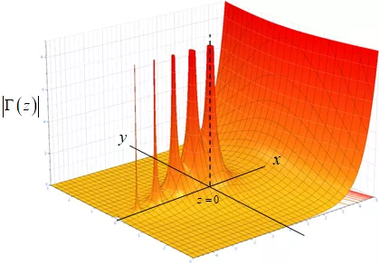
Plot of Gamma Function
Plot of Gamma Function
18
N
o
t
e
:
T
h
e
r
e
a
r
e
s
i
m
p
l
e
p
o
l
e
s
a
t
z
=
0
,
-
1
,
-
2
,
…
Plot of Gamma Function (cont.)
Plot of Gamma Function (cont.)
19
(
x
)
and 1 /
(
x
)
In fact,
1 /
(
z
)
is analytic everywhere.
N
o
t
e
:
(
x
)
n
e
v
e
r
g
o
e
s
t
o
z
e
r
o
.
Asymptotic Form of Gamma Function
Asymptotic Form of Gamma Function
20
Sterling’s formula (asymptotic series for large argument):
Taking the ln of both sides, we also have
The Gamma function is a versatile mathematical function that generalizes the factorial function to non-integer and complex values. It has various integral definitions such as the Euler-integral form. The proof of the factorial property of the Gamma function is demonstrated through analytical continuation. Equivalence between different integral forms is explored, showcasing the interconnectedness of these representations.

Download Presentation

Please find below an Image/Link to download the presentation.
The content on the website is provided AS IS for your information and personal use only. It may not be sold, licensed, or shared on other websites without obtaining consent from the author.If you encounter any issues during the download, it is possible that the publisher has removed the file from their server.
You are allowed to download the files provided on this website for personal or commercial use, subject to the condition that they are used lawfully. All files are the property of their respective owners.
The content on the website is provided AS IS for your information and personal use only. It may not be sold, licensed, or shared on other websites without obtaining consent from the author.
E N D
Presentation Transcript
ECE 6382 ( ) z y x z = 0 Fall 2023 David R. Jackson Notes 14 The Gamma Function Notes are from D. R. Wilton, Dept. of ECE 1
The Gamma Function The Gamma function appears in many expressions, including Bessel functions, etc. It generalizes the factorial function n! to non-integer values and even complex values. It appears in the method of steepest descent (a method for obtaining the asymptotic expansion of a class of integrals). 2
Definition 1 Definition # 1 1 2 3 1)( z n z 0, 1, 2, ( ) z lim n , n z + + + ( 2) ( ) z z z n This definition gives the Gamma function a nice property for z = n (a positive integer), as proven on the next slide: ( ) = ( ) n 1 ! n (factorial property) 3
Definition 1 (cont.) Proof of factorial property: 1 2 3 1)( z n z 0, 1, 2, ( ) z lim n , n z + + + ( 2) 1 2 3 z + ( ) z z z n n z nz n + 1 z + = = ( 1) lim n ( ) lim z z n + + + = + + ( 1)( 2) ( + 1) ( 1) z n z n ( 1) ( ) z z z 1 2 3 (4) n n = = = = Note that , and (1) lim n 1 (2) 1 (1) 1, n + 1 2 3 ( (3) 1) = n = 2 1, = = = 4 3 2 1, = (3) 2 (2) 3 3 2 1, (5) 4 (4) . etc Hence ( ) + = ( 1) ! = n n ( ) n 1 ! n or n = n = 0,1,2, 1,2,3 4
Definition 2 Definition # 2 1 t z ( ) z , Re 0 e t dt z 0 This is the Euler-integral form of the definition. Note: Leonard Euler ( ) ( ) iy 1 1 1 1 z x x x = = = ln ln iy t iy t t t t t e t e 1 1 z x = 0 t t x for the integral to converge at = 0 t Note: Definition 1 is the analytic continuation of definition 2 from the right-half plane into the entire complex plane (except at zero and the negative integers). 5
Equivalent Integral Forms The following three integral definitions are all equivalent: 1 t z ( ) z , Re 0 e t dt z 0 2 2 1 2 s z = = (let ) ( ) z 2 , Re 0 e s ds z t s 0 1 z 1 1 s ( ) = = (let ) ( ) z ln , Re 0 ln 1/ ds z t s 0 6
Equivalence of Definitions 1 and 2 Equivalence of definitions #1 and #2 n t n t Use , lim 1 n e n n t n ( ) z 1 1 z t z = Define ( , ) F z n 1 ; ( , ) F z n t dt e t dt 2 0 0 n t n = Letting and integrating by parts t imes , w n Factor appearing in Definition #1 ( ) + 1 1 1 2 3 1)( + 1 z n n n ( ) z n + 1 1 z z z = = ( , ) F z n 1 n w w dw n w dw + ( 2) ( 1) z z z n 0 0 1 + = Hence lim ( , n ) ( ) z F z n z n 1 (Please see next slide.) 1 2 3 1)( z n z 0, 1, 2, ( ) z lim n , n z 1 + + + ( 2) ( ) z z z n 7
Equivalence of Definitions 1 and 2 (cont.) Integration by parts development: 1 n ( ) 1 z 1 I w w dw 0 dv dw u Integrate by parts once: 1 1 z z w w 1 n n ( ) ( ) = 1 1 I w n w dw z z 0 0 1 z w 1 n ( ) = + 0 1 n w dw z 0 1 n z 1 n ( ) z = 1 w w dw 0 8
Equivalence of Definitions 1 and 2 (cont.) 1 n ( ) 1 z Integrate by parts twice: 1 I w w dw 0 dv dw 1 u n z 1 n ( ) z = 1 I w w dw 0 1 1 + + 1 1 z z n z w z n z w z 1 2 n n ( ) ( )( ) ( ) = 1 1 1 1 w n w dw + + 1 1 0 0 ( ( ) ) 1 + 1 1 n n z z 2 n ( ) + 1 z = + 0 1 w w dw 0 ( ( ) ) 1 + 1 1 1 n n z z 2 n ( ) + z n + 1 z 1 = 1 w w dw w dw 0 0 After n times: ( )( z ) + 1 1 2 3 2 1 n n n z z n ( ) z n + n n 1 = 1 I w w dw + + ( 1)( 2) ( 1) z 0 9
Definition 3 Definition # 3 The Weierstrass product form can be shown to be equivalent to definitions #1 and #2. z n 1 ( ) z z n z = + 1 ze e = 1 n = where is the Euler -Mascheroni constant. 0.5772156619 10
Euler Reflection Formula Euler Reflection Formula ( ) (1 z = ) z (Proof omitted.) y sin z x = 1/ 2 z Geometric interpretation of reflection formula: In the horizontal direction, the two points are reflections about the x = 1/2 line. ( ) 1 1/ 2 1/ 2 x x x 1 1 z z Note: We can use this formula along with definition #2 to find (z) for Re(z)< 0. 1 = 0, 1, 2, ( ) z , Re 0, z z sin (1 ) z z 11
Euler Reflection Formula (cont.) A special result that occurs frequently is (1/2). To calculate this, use the reflection formula: ( ) (1 z = ) z sin z Set z = 1/2: = (1/2) 12
Summary of Factorial Properties Summary of Factorial Generalization ( )( ) ( )( )( ) 3 2 1 = ! 1 2 n n n n Integers 1,2,3 n = ( ) = Real numbers x t x = + ! 1 x x e t dt 1 0 ( ) Complex numbers ( ) Re z = t z = + ! 1 z z e t dt 1 0 13
Summary of Factorial Properties (cont.) Summary of Factorial Generalization (cont.) ( ) ( ) t z = + = ! 1 Re 1 z z e t dt z 0 Complex numbers z + 1, 2 1 = ( ) z sin (1 ) z z 14
Pole Behavior Simple poles of (z) are at n = 0, -1, -2, -3, + = = ( 1) ( ) z & (1) 1 z z Recall: (z) has simple pole at z = 0 Residue = 1 Use + ( 1) z + = = ( 1) ( ) z ( ) z z z z + + ( 2) 1 z ( ) + = + + + = ( 2) 1 ( 1) ( 1) z z z z z + + + + ( 2) 1 2) 1 z = ( ) z z (z) has simple pole at z = -1 Residue = -1 z ( z = ( ) z ( ) z z 15
Pole Behavior (cont.) + ( z 3) 2 ( z z z ( ) + = + + + = ( 3) 2 ( 2) ( 2) z z z z + + 3) 2 (z) has simple pole at z = -2 Residue = +1/2 ( )( ) 1 + = ( ) z z z + + + ( 3) z z = ( ) z ( )( ) + 1 2 z z + ( z 4) 3 z ( ) + = + + + = ( 4) 3 ( 3) ( 3) z z z z + + ( z 4) 3 z ( )( )( ) 1 (z) has simple pole at z = -3 Residue = -1/6 + + = 2 ( ) z z z z + + + ( 4) 2 z z = ( ) z ( )( )( ) + + 1 3 z z z 16
Pole Behavior (cont.) Residues at Poles In general (after n+1 steps), we will have: (z) has simple pole at z = -n + + ( 1) 3 z n z = ( ) z ( )( )( ) ( ) + + + + 1 2 z z z z n ( ) + + + ( z 1) 3 n n ( ) z ( ) = + Res Lim z z n ( )( )( ) ( ) + + + = z n 1 2 z z z z n n 1 z = ( )( )( 1 ) ( ) + + + + 1 2 3 1 z z z z n Hence = z n = ( ) 1 ! n n ( )( ) ) ( )( )( ) + 1 3 2 1 n n ( ) z = Res ( = z n n 1 = ( )( n ) ( )( )( ) 3 2 1 1 n 17
Plot of Gamma Function ( ) z y x z = 0 ( ) 1 ! n n ( ) z = Res Note: There are simple poles at z = 0, -1, -2, = z n 18
Plot of Gamma Function (cont.) (x) and 1 / (x) Note: (x) never goes to zero. In fact, 1 / (z) is analytic everywhere. 19
Asymptotic Form of Gamma Function Sterling s formula (asymptotic series for large argument): + + z as 2 1 1 139 571 ( ) z + z z 1 z e 2 3 4 12 288 51840 2488320 z z z z z w Taking the ln of both sides, we also have 1 2 1 1 1 z ( ) z + + + ln ln ln z z z 3 5 2 12 360 1260 z z z 2 3 w w ( ) + = + Note: ln 1 w w 2 3 20


")


")
")


")

")

")
")

")