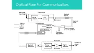
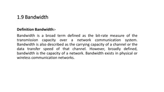
Understanding Bandwidth and Dispersion in Fiber Optic Communication
This presentation provides a comprehensive overview of bandwidth and dispersion in fiber optic communication. It covers essential terminologies like microns, nanometers, millimeters, and dB, explaining concepts such as bandwidth capacity, dispersion cancellation, and modal bandwidth in multimode fibers. The discussion extends to single-mode fiber dispersion, including waveguide dispersion and material dispersion factors.

Download Presentation

Please find below an Image/Link to download the presentation.
The content on the website is provided AS IS for your information and personal use only. It may not be sold, licensed, or shared on other websites without obtaining consent from the author. Download presentation by click this link. If you encounter any issues during the download, it is possible that the publisher has removed the file from their server.
E N D
Presentation Transcript
Presentation Title Goes Here Bandwidth vs. Dispersion, or A Light Refresher of Fiber Optic Terminology
2 What Does It All Mean? A Light Refresher of FO Terminology Bandwidth, Dispersion Microns, Nanometers, Millimeters, Mils dB, Attenuation Low Water Peak, Zero Water Peak Modes, Rays Core Diameter, Mode Field Diameter Analog, Digital
3 Bandwidth and Dispersion Bandwidth (MBA Jargon): ability to do additional work; generally used to indicate that speaker cannot or would not prefer to do additional work, as in: I don t think I ll have any bandwidth this Friday Dispersion (Lingo): You can t cast dispersion, but you can cancel it out (and it s not nice to cast aspersions either)
4 Bandwidth of Multimode Fibers The information carrying capacity of the fiber, bandwidth is the frequency at which the received signal drops to half of its transmitted level (-3dB) BDP - Bandwidth of a fiber multiplied by the length of the fiber (MHz-Km) Example: ALE Fiber (50 m 10Gig) BDP of 4700 MHz- km @ 850nm 1 km of the fiber would have a bandwidth of 4700 MHz 2 km of the fiber would have a bandwidth of 2350 MHz 4 km of the fiber would have a bandwidth of 1175 MHz 8 km of the fiber would have a bandwidth of 588 MHz
OCC Laser Bandwidth Comparison Effective Modal Bandwidth of OCC Multimode Products 5000 4700 4500 OM4 - ALE 4000 OM3 - ALT 3500 OM2+ - ALX 3000 OM2 - ALS MHz-km 2500 OM1 - WLX 2000 2000 OM1 - WLS 1500 950 1000 510 500 500 500 500 500 500 385 500 220 0 850 nm 1300 nm
6 Dispersion in Single-mode Fiber Dispersion is a measure of the pulse spreading in an optical fiber, limiting information capacity Single-mode material dispersion happens when different wavelengths propagate at different speeds, even from a single laser
7 What Causes Dispersion in Single-mode Fiber? Single-mode dispersion is the result of: 1.Waveguide dispersion - optical energy travels in both the core & cladding at slightly differ speeds 2.Material dispersion (predominant factor of single-mode Dispersion) glass s index of refraction changes with and this causes different s to travel at different speeds Zero-Dispersion Wavelength is the wavelength or wavelengths at which the material dispersion and waveguide dispersion cancel one another.
Zero-Dispersion Wavelength Most SM fibers (SLS, SLX, SLA, and SLB) have zero dispersion point at 1310 nm Typical value for SLX and SLA fibers 0.088 ps/nm2-km
9 Numbers, Large and Small
10 Numbers Fun Facts Optical fibers are measured in metric units Nanometers and microns (1300 nm = 1.3 microns) Microns and millimeters (900 microns 0.9 mm) Cable parameters may be in English or metric units Feet vs. meters has forever been a source of errors in fiber optics don t let it happen to you! Tensile loading may be quoted in lbs-f or Newtons Jacket thickness is often measured in mils
Attenuation (or Power Loss) Logarithmic decibel ratio of optical power output to power input in a fiber optic system Input Power (dBm) P1 Output Power (dBm) P2 Optical Loss = P1-P2 (dB) Note: dBm is the actual power level represented in milliwatts dB is the difference between the powers
12 Why use Decibels? A very large range of numbers can be represented by a convenient number Clearly visualize huge changes of some quantity The overall decibel loss of a multi-component system can be calculated simply by summing the decibel loss of the individual components Fiber and connector losses simply add together The human perception of the intensity of sound or light is more nearly proportional to the logarithm of intensity than to the intensity itself
How Much Optical Power is Lost? dB Power Out as a % of Power In % of Power lost Remarks 1 79% 21% - 2 63% 37% - Every 3 dB, the power is lost 3 1/2 the Power 50% 50% 4 40% 60% - 5 32% 68% - Every 10 dB, 90% of the power is lost 25% 75% 1/4 the Power 6 7 20% 80% 1/5 the Power 8 16% 84% 1/6 the Power 12% 88% 1/8 the Power 9 10 10% 90% 1/10 the Power 11 8% 92% 1/12 the Power 6.3% 93.7% 1/16 the Power 12 20 1% 99% 1/100 the Power 30 0.1% 99.9% 1/1,000 the Power 40 0.01% 99.99% 1/10,000 the Power
Optical Fiber Attenuation Spectrum 5 Water Peak 4 Caused by water absorption (OH-) Attenuation (dB/km) 1st Window 3 2nd 3rd Window Window 2 Operating Bands O E S C L U 1 Secondary Water Peaks 0 700 800 900 1000 1100 1200 1300 1400 1500 1600 1700 Wavelength - (nm)
15 Low Water Peak vs. Zero Water Peak Wavelength (nm)
16 What are those modes, Anyway? Optical energy travelling along a fiber is contained by the core/cladding boundary The geometry of the fiber, refractive index, and wavelength of light constrain the light energy to exist in certain discrete physical patterns called modes The larger the core in wavelengths, the more modes which can exist Single-mode fiber becomes dual-mode around 1260 nm
17 Just what are those modes, Anyway? Finite number of EM field distributions in the FO core
18 Mode Field Diameter For single-mode some light travels in the cladding (around 10+%) Mode Field Diameter varies with wavelength At 1310 nm 8.8 to 9.2 micron typical At 1550 nm 10.2 to 10.5 micron typical
19 Analog vs. Digital Analog means analogous, or a like representation of something else Analog implies continuous change and infinite levels Analog sound is a representation of vibration and varies continuously over a wide range AM radio is analog because the strength of the radio signal varies just like the strength of a sound signal Digital means having discrete levels and finite values Our hands have 10 digits, not 3.14159265 digits Morse Code is digital because it is a sequence of on or off timed pulses Digital usually requires some form of computing power
20 Early Digital Computer
21 Analog Computer
22 Light Signals may be Digitally Encoded Example of light transmission of digital information
23 Digital vs. Analog If the signal is just above the noise threshold, digital gives a more faithful reproduction of the input Analog transmits the noise just like the signal Digital is either on or off, so noise is rejected once the receiver makes the correct on/off decision Digital encoding may feature error detection and correction algorithms Digital requires some form of computing power Processors needed for encoding and decoding the signal The faster the processors and communications channel, the more information which can be transmitted
24 A Light Refresher on Fiber Optics Terminology Questions?


")