Percentile Based Test of Location Parameter & Unbiased Estimates
Proposing a new percentile-based test for determining the true mean of a normal distribution when two symmetric sample percentile values are known. The test statistic is explored for its distribution properties and performance through simulation. Additionally, investigating unbiased estimates and identifying the best percentile pair for estimating parameters.
Download Presentation

Please find below an Image/Link to download the presentation.
The content on the website is provided AS IS for your information and personal use only. It may not be sold, licensed, or shared on other websites without obtaining consent from the author. Download presentation by click this link. If you encounter any issues during the download, it is possible that the publisher has removed the file from their server.
E N D
Presentation Transcript
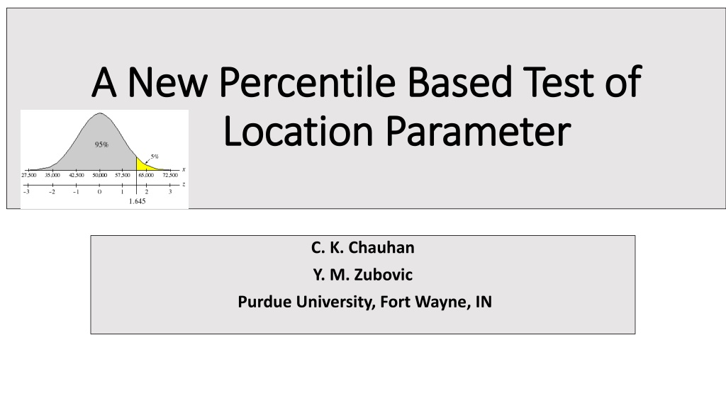
A New Percentile Based Test of A New Percentile Based Test of Location Parameter Location Parameter C. K. Chauhan Y. M. Zubovic Purdue University, Fort Wayne, IN
Traditional t test Traditional t test H H 0: 0 1: 0 A random sample of n observations has a mean and standard deviation of S. Reject if 0 H n X ( ) X 0 t ( 1) n s
Sometimes only Sometimes only two symmetric two symmetric percentile values are given percentile values are given When designing doors and desks, the 5thand 95thpercentiles of sitting and standing heights are commonly recorded. A study on SAT scores may only report 75thand 25thpercentile values. In studies of noise level reduction in hearing protection devices 20thand 80th percentiles may be recorded. Only the minimum/maximum temp values of a given day may be recorded.
Introduction Introduction We propose a test for the true mean, , of a normal distribution when only two symmetric sample percentile values are known. The proposed test statistic has an asymptotic normal distribution. However for small values of n, it doesn t fit any known distribution. The distribution of the proposed test statistic is explored via simulation. The power and the robustness of the proposed test are under revision. The proposed test is easy to use and performs well, especially the one based on 75th and 25thpercentile values as well as 80thand 20thpercentile values.
Objectives Objectives Primary Objective: Develop a percentile based test and investigate its properties. Secondary objective: Find percentile based unbiased estimates of and and investigate which percentile pair provides the best estimates of these parameters.
Notation Notation Normal distribution with mean and standard deviation , both unknown. Let f and F, denote respectively, the density function and cumulative distribution function of a standard normal. Let be the kthpercentile value, where is defined the same way. Let be the sample percentiles (symmetric ) obtained from n values. It is known that the asymptotic distribution of is normal with mean and ( ). p kP 1( /100) k = + kP F = lP 0 100, 100 , k l l k p p , l k lP lp l
Percentile Percentile Based Unbiased Estimates of and Based Unbiased Estimates of and Since 1( /100) k = + kP F = + ( )/ 2 p p It follows that l k = ( )/ p p w , l k l n where is such that E( )= , l n w
The Proposed Test Statistic The Proposed Test Statistic H 1: 0 ( ) 0 Consider U= ( ) stddev where estimates of and , are defined as before. Note : is a linear combination of two sample percentiles. Only the asymptotic formulas for the variance /covariance of are available. For greater accuracy ( specially for small n) the values of the standard deviation of were obtained via simulation. p p , l k
Variance Variance Covariance formulas Covariance formulas 2 *(1 nf *) ( *)) k k k = 2 ( ) p k 2 1 ( F 2 *(1 *) k l = * /100 k k = cov( , ) p p k l + 1 1 ( 2) ( ( *)) ( k ( *)) l n f F f F
= ( )/ p p w unbiased estimate of unbiased estimate of : Values of : Values of divisor divisor give below : give below : , l k l n Percentile Pair n 95, 5 90,10 80,20 75,25 max,min 10 3.0770 2.9670 1.8778 1.4800 3.0744 15 20 3.4740 3.6670 2.8820 2.7490 1.8106 1.7706 1.4214 1.4076 3.4590 3.7280 25 3.6610 2.7240 1.755 1.3940 3.9270 30 3.6206 2.6990 1.7432 1.3844 4.0922 40 3.4672 2.6478 1.7260 1.3818 4.3278 50 3.4644 2.6300 1.7166 1.3788 4.5142 75 3.3998 2.6098 1.7086 1.3636 4.8222 100 3.3630 2.6006 1.7002 1.3626 5.0310 150 3.3370 2.5896 1.6962 1.3576 5.3030 200 3.3226 2.5826 1.6928 1.3562 5.5006 250 3.3150 2.5788 1.6918 1.3534 5.6462 300 3.3120 2.5748 1.6868 1.3544 5.7598
Simulated values of standard deviations of given below Simulated values of standard deviations of given below ( l p = + )/ 2 p k Percentile Pair X n 95, 5 90, 10 80, 20 75,25 max, min 10 0.4430 0.4126 0.3436 0.3333 0.4326 .3162 15 0.3936 0.3119 0.2852 0.2885 0.3965 .2582 20 0.3684 0.2849 0.2504 0.2429 0.3813 .2236 25 0.3159 0.2552 0.2136 0.2188 0.3657 .2000 30 0.2771 0.2367 0.2052 0.1994 0.3552 .1826 40 0.2432 0.2022 0.1790 0.1740 0.3404 .1581 50 0.2157 0.1810 0.1593 0.1588 0.3353 .1414 75 0.1775 0.1443 0.1295 0.1301 0.3147 .1155 100 0.1531 0.1264 0.1136 0.1109 0.3069 .1000 150 0.1257 0.1048 0.0916 0.0911 0.2903 .0816 200 0.1080 0.0893 0.0802 0.0790 0.2815 .0707 250 0.0956 0.0791 0.0715 0.0718 0.2794 .0632 300 0.0876 0.0722 0.0657 0.0628 0.2755 .0577
Which percentile pair provides the best unbiased estimate of Which percentile pair provides the best unbiased estimate of simulated values of Standard deviation of given below simulated values of Standard deviation of given below n 95,5 90,10 80,20 75,25 max,min s 10 0.2534 0.2570 0.2831 0.3097 0.2592 0.2320 15 0.2172 0.1957 0.2437 0.2891 0.2167 0.1876 20 0.1900 0.1872 0.2163 0.2448 0.1935 0.1616 25 0.1637 0.1643 0.1978 0.2162 0.1810 0.1446 30 0.1506 0.1533 0.1786 0.2039 0.1692 0.1320 40 0.1388 0.1387 0.1563 0.1771 0.1547 0.1136 50 0.1194 0.1211 0.1432 0.1620 0.1442 0.1016 75 0.0998 0.1011 0.1184 0.1366 0.1285 0.0824 100 0.0880 0.0865 0.1043 0.1138 0.1210 0.0714 150 0.0713 0.0730 0.0845 0.0947 0.1099 0.0583 200 0.0619 0.0637 0.0727 0.0813 0.1031 0.0506 250 0.0558 0.0561 0.0648 0.0733 0.0984 0.0451 300 0.0505 0.0510 0.0603 0.0680 0.0949 0.0410
( ) Critical Values of the Proposed Test Statistic at = .01, .025, .05, .10 0 ( ) stddev n alpha U95 U90 U80 U75 Urange ts 10 0.010 2.41971 2.52207 2.87747 3.06681 2.47567 2.82548 10 0.025 2.02490 2.10807 2.27295 2.34767 2.07173 2.22849 10 0.050 1.67284 1.73075 1.84227 1.86542 1.71153 1.81187 10 0.100 1.28993 1.33380 1.39905 1.39051 1.31976 1.38818 15 0.010 2.38973 2.58164 2.78513 2.89290 2.36183 2.72835 15 0.025 2.03826 2.12215 2.17501 2.27377 2.01446 2.18429 15 0.050 1.69582 1.76037 1.75871 1.80392 1.67602 1.77464 15 0.100 1.33053 1.36834 1.33470 1.32593 1.31499 1.34380 20 0.010 2.29382 2.41401 2.59745 2.69564 2.27624 2.50296 20 0.025 1.90767 2.06397 2.10221 2.17593 1.88845 2.08475 20 0.050 1.63647 1.70549 1.71910 1.76880 1.61671 1.70007 20 0.100 1.28127 1.32110 1.32304 1.32249 1.27211 1.32372 25 0.010 2.30263 2.31669 2.61551 2.65369 2.19910 2.52047 25 0.025 1.96000 1.92463 2.13280 2.09582 1.88477 2.04502 25 0.050 1.62035 1.58302 1.73862 1.69329 1.60271 1.69204 25 0.100 1.28442 1.22927 1.34899 1.27984 1.26297 1.30420 30 0.010 2.36864 2.35344 2.53327 2.58735 2.26386 2.45234 30 0.025 1.98301 1.97175 2.03282 2.09925 1.94184 2.04476 30 0.050 1.69355 1.64275 1.67195 1.71382 1.64330 1.69438 30 0.100 1.29339 1.27951 1.30610 1.32206 1.27121 1.29768 40 0.010 2.41469 2.37692 2.39961 2.46769 2.25728 2.38810 40 0.025 2.06068 1.98741 1.98492 2.06428 1.90580 2.00390 40 0.050 1.72464 1.68844 1.67742 1.72844 1.63085 1.70901 40 0.100 1.35238 1.29447 1.30387 1.33656 1.26765 1.32826 50 0.010 2.37557 2.37411 2.47978 2.41818 2.24311 2.52664 50 0.025 1.98785 1.96964 2.03257 2.07531 1.89203 2.07995 50 0.050 1.65226 1.65182 1.69724 1.68710 1.59013 1.69570 50 0.100 1.29365 1.29920 1.29806 1.28084 1.24784 1.31369 75 0.010 2.37435 2.37946 2.45801 2.43590 2.23682 2.41253 75 0.025 1.95639 1.99835 2.04473 2.03659 1.91648 2.01927 75 0.050 1.66512 1.70153 1.68189 1.67615 1.59485 1.67033 75 0.100 1.29547 1.33182 1.32640 1.31553 1.25271 1.31139 100 0.010 2.32506 2.32839 2.33481 2.44156 2.23511 2.36436 100 0.025 1.98473 1.97436 1.96112 2.01160 1.93400 1.99198 100 0.050 1.66572 1.64537 1.64281 1.67295 1.63687 1.66557 100 0.100 1.30150 1.29744 1.27368 1.29650 1.29650 1.29616
Partial Table of the Critical Values of U. Partial Table of the Critical Values of U. n U95 U90 U80 U75 Urange 10 0.010 2.41971 2.52207 2.87747 3.06681 2.47567 10 0.025 2.02490 2.10807 2.27295 2.34767 2.07173 10 0.050 1.67284 1.73075 1.84227 1.86542 1.71153 10 0.100 1.28993 1.33380 1.39905 1.39051 1.31976
S Simpler Format of the Proposed Test : impler Format of the Proposed Test : : H 1 0 Reject if U= >C 0 H ( ) 0 ( ) stddev + + (.5 .5 B ) (.5 .5 ) )/ p p p p p = 0 0 l k l k C ( B p w l k C p C p = + + ' / C CB W (.5 ) (.5 ) 0 l k C p C p + + (.5 ) (.5 ) 0 l k
C p C p + + (.5 ) (.5 ) Critical region : Critical region : 0 l k The values of C are available for Percentile pair: (95, 5 ) (90, 10) (80, 20 ) (75, 25) (max, min) n= 10, 20, 25, 30, 40, 50, 60 , 75, 100 = .01, .025, .05, .10 For n> 100, the distribution of U approaches normal
1: 50 H Example Example Suppose based on 40 values from a normal distribution, the 95th and 5th values are 37.5 and 72.8 respectively. = (.5 C p = = + = (37.5 (72.8 37.5)/3.4672 ( ) .2432 stddev 72.8)/ 2 55.1 = 10.18 2.4757 C p + + ) (.5 ) 0 l k Reject null hypothesis if + + (.5 .1209715) .379 l p + (.5 .1209715) 50 p p 0 l k .62097 p k Since {.379(37.5) + .62097(72.8)} is greater than 50, we reject the null hypothesis.
Properties of the Proposed Test : under revision Properties of the Proposed Test : under revision Power of the test : P( rejecting the null , given is true) : HIGH H 1 Robustness of the test : A robust test is resistant to errors in the results ( performs well when the assumption of normality fails).
Size and the Power of the proposed Size and the Power of the proposed test. Assume test. Assume = 0 0 t Eff(80) Eff(75) n / 0.00 0.25 0.50 0.75 1.00 95,5 90,10 80,20 75,25 max,min 4.8 18.4 41.9 69.8 89.6 10 3.1 10.9 25.5 45.4 65.6 3.7 12.4 28.2 49.3 69.8 4.4 15.8 34.4 59.8 81.1 4.3 15.0 33.4 59.1 80.2 3.4 11.5 26.5 46.7 66.6 85.9 82.1 85.7 90.5 81.5 79.7 84.7 89.5 5.1 23.8 57.5 86.4 98.0 15 0.00 0.25 0.50 0.75 1.00 4.0 14.0 32.3 56.3 76.6 4.8 18.8 44.4 72.3 90.4 4.2 19.6 47.4 76.0 93.0 4.0 17.4 43.1 71.6 91.0 3.9 13.7 31.6 55.6 76.1 82.4 82.4 88.0 94.9 73.1 75.0 82.9 92.9 5.1 28.9 70.1 94.1 99.7 20 0.00 0.25 0.50 0.75 1.00 4.2 14.9 36.7 61.7 82.1 4.7 19.9 51.1 79.5 94.6 4.5 23.2 58.2 86.9 97.9 4.6 23.3 57.6 87.1 97.9 4.0 14.1 35.1 59.7 80.2 80.3 83.0 92.3 98.2 80.6 82.2 92.6 98.2 5.2 33.1 77.9 97.7 99.9 25 0.00 0.25 0.50 0.75 1.00 4.6 17.5 45.6 74.2 91.5 4.1 22.6 58.9 88.0 98.1 5.1 29.1 69.4 94.5 99.5 4.5 27.0 66.5 93.6 99.4 3.9 14.0 37.1 63.4 83.4 87.9 89.1 96.7 99.6 81.6 85.4 95.8 99.5
= Size and the Power of the proposed Size and the Power of the proposed test: test: 0 0 t Eff(80) Eff(75) n / 0.00 0.25 0.50 0.75 1.00 95,5 90,10 80,20 75,25 max,min 4.8 18.4 41.9 69.8 89.6 10 3.1 10.9 25.5 45.4 65.6 3.7 12.4 28.2 49.3 69.8 4.4 15.8 34.4 59.8 81.1 4.3 15.0 33.4 59.1 80.2 3.4 11.5 26.5 46.7 66.6 85.9 82.1 85.7 90.5 81.5 79.7 84.7 89.5 5.1 23.8 57.5 86.4 98.0 15 0.00 0.25 0.50 0.75 1.00 4.0 14.0 32.3 56.3 76.6 4.8 18.8 44.4 72.3 90.4 4.2 19.6 47.4 76.0 93.0 4.0 17.4 43.1 71.6 91.0 3.9 13.7 31.6 55.6 76.1 82.4 82.4 88.0 94.9 73.1 75.0 82.9 92.9 = 0 0 5.1 28.9 70.1 94.1 99.7 20 0.00 0.25 0.50 0.75 1.00 4.2 14.9 36.7 61.7 82.1 4.7 19.9 51.1 79.5 94.6 4.5 23.2 58.2 86.9 97.9 4.6 23.3 57.6 87.1 97.9 4.0 14.1 35.1 59.7 80.2 80.3 83.0 92.3 98.2 80.6 82.2 92.6 98.2 5.2 33.1 77.9 97.7 25 0.00 0.25 0.50 0.75 4.6 17.5 45.6 74.2 4.1 22.6 58.9 88.0 5.1 29.1 69.4 94.5 4.5 27.0 66.5 93.6 3.9 14.0 37.1 63.4 87.9 89.1 96.7 81.6 85.4 95.8
Robustness of the Proposed Test: Under revision Robustness of the Proposed Test: Under revision N / Distribution 95,5 90,10 80,20 75,25 max,min t 10 0 Uniform Laplace 1 9 1.2 9.5 3.3 7.3 4.0 5.2 1.1 9.3 4.7 5.2 0.25 Uniform Laplace 4.0 18.7 4.7 20.2 9.6 24.1 10.9 22.7 4.2 19.4 16.7 20.8 0.5 Uniform Laplace 13.9 34.2 16.2 36.6 23.7 48.2 23.7 50.1 14.7 35.0 39.1 47.8 0.75 Uniform Laplace 38.5 51.2 46.1 54.4 46.3 70.9 43.5 74.2 40.8 52.0 68.7 73.9 1 Uniform Laplace 91.0 64.5 94.4 68.0 76.8 84.9 68.3 88.2 92.4 65.2 90.7 88.7 15 0 Uniform Laplace 0.5 11.1 1.1 11.0 3.0 7.6 3.9 5.6 0.4 10.8 5.1 4.8 0.25 Uniform Laplace 3.2 21.9 7.9 26.6 12.4 29.8 12.0 28.2 3.0 21.5 22.7 25.7 0.5 Uniform Laplace 19.0 38.2 37.2 48.5 32.3 60.4 27.9 61.2 18.1 37.6 54.9 60.6 0.75 Uniform Laplace 84.5 54.9 91.8 69.2 66.4 83.5 54.2 84.4 82.6 54.4 87.0 86.0 1 Uniform Laplace 99.9 69.4 100.0 84.3 94.7 94.2 83.0 94.7 99.9 69.0 98.9 96.6 20 0 Uniform Laplace 0.1 12.0 0.7 11.5 2.5 7.7 3.6 6.8 0.1 11.7 4.8 5.2 0.25 Uniform Laplace 2.5 23.8 8.0 29.9 13.2 35.5 14.6 37.4 2.1 23.1 27.2 31.2 0.5 Uniform 25.9 43.3 42.3 40.2 22.6 68.6
References: Arnold, B.C., Balakrishnan, N., Nagaraja, H.N. (2008). A First Course in Order Statistics. Philadelphia: SIAM. Benson, F. (1949). A Note on the Estimation of Mean and Standard Deviation from Quantiles. Journal of the Royal Statistical Society, B 11:91-100. David, H. (1954). The Distribution of Range in Certain Non-Normal Populations. Biometrika 41:463- 468. Ogawa, J. (1951). Contributions to the theory of systematic statistics, I. Osaka Mathematical Journal 3:175-213. Patnaik, P.B. (1950). The Use of Mean Range as an Estimator of Variance in Statistical Tests. Biometrika 37:78-87. Rhiel, S. (1989). An Improved Range Estimator of Sigma for Determining Sample Sizes. Communications in Statistics. Simulation and Computation 18:1295-1309. Sarhan, A.E., Greenberg, B.C. (1962). Contributions to Order Statistics. New York: Wiley.
