Exploring EViews Data Functions for Data Manipulation
EViews offers a wide range of built-in functions for data manipulation, including generating random numbers, statistical functions, and time series functions. This tutorial provides examples of how to utilize these functions within EViews to perform various data operations effectively.

Download Presentation

Please find below an Image/Link to download the presentation.
The content on the website is provided AS IS for your information and personal use only. It may not be sold, licensed, or shared on other websites without obtaining consent from the author. Download presentation by click this link. If you encounter any issues during the download, it is possible that the publisher has removed the file from their server.
E N D
Presentation Transcript
EViews Training Data Objects: Data Functions Note: Information for examples in this tutorial can be found in these files. Data: Data.xlsx Results: Results.wf1 Practice Workfile: Data.wf1
Data and Workfile Documentation Data.wf1 and Data.xlsx have the following data: Workfile Page: Timeseries (Data.xlsx tab Timeseries): quarterly, Q1 1980 Q1 2012 GDP real GDP data (billions of dollars) from the Bureau of Economic Analysis. PCE real consumption data (billions of dollars) from the Bureau of Economic Analysis. Inv real private sector investments (billions of dollars) from the Bureau of Economic Analysis. G real government spending (billions of dollars) from the Bureau of Economic Analysis. y a series that grows over time (trend series). 2
Data Functions EViews has a large number of built-in functions that allow you to perform data manipulation. EViews functions are typically denoted by the symbol @ . This tutorial reviews some typical functions used for data manipulation, such as: Random numbers Statistical Functions Commonly Used Time Series Functions 3
Generating Random Numbers (Series): Example 1 You can generate a series of (pseudo) random numbers drawn from a variety of distributions. There are a number of ways to generate a random series. Generating a random series: Example 1 1. Open EViews workfile Data.wf1. 2. Select Quick Generate Series from the main menu. 3. Type y1 = nrnd in the dialog box and press Enter. 5
Generating Random Numbers (Series): Example 1 (cont d) The result is shown here. As seen, this generates a series y1, which is normally distributed with mean 0 and standard deviation equal to 1. 6
Generating Random Numbers (Series): Example 2 Alternatively, you can create a random series by typing in the command window. Generating a random series: Example 2 Type in the command window: 1. series z=nrnd Press Enter. 2. This creates a new series z, which is normally distributed with mean 0 and standard deviation equal to 1. 7
Generating Random Numbers (Series): Example 3 Suppose you want to simulate a random walk process with distribution properties similar to the observed distribution of an existing series (for example, gdp): Generating a random series: Example 3 Type in the command window: 1. 2. smpl @all series newdata = 0 smpl 1980q2 @last newdata=newdata(-1)+@mean(d(gdp))+@stdev(d(gdp))*nrnd Press Enter after each command line. Note: for an explanation of statistical functions @mean, @stdev, or d(gdp), see Descriptive Statistics in this tutorial. 8
Generating Random Numbers (Series): Example 3 (cont d) Here we show both the new series (newdata) and the GDP series. As seen, the command has generated a series newdata, which follows the same distribution process as the gdp series. Note that the commands instruct EViews to first create a new series (newdata) consisting of zeros. Then, from the second observation (1980q2) onwards it sums the preceding observation with the mean and standard deviation of differenced gdp (multiplied by a normal random variable). 9
Generating Random Numbers (Series): Common Functions/Commands EViews has a number of functions/commands that allow you to draw from a variety of distributions. The most commonly used functions/commands are summarized below. Common Commands/Functions Function/Command Description Normal distribution (mean 0, st. dev. 1) series y=nrnd or (y=@rnorm) Normal distribution (mean 3, variance 4) series y=3+@sqr(4)*nrnd Lognormal distribution (mean=1, st. dev 4) series y=@rlognorm(1,4) Uniform distribution on (1,3) series y=@runif(1,3) Uniform distribution on (0,1) series y=rnd Uniform distribution on (1,3) (same as @runif(1,3)) series y=1+(3-1)* rnd Fills series y with random integers drawn randomly from 0 to 100 series y=rndint(0,100) 10
Generating Random Numbers (Series): PDF and CDF It is also very easy to generate the pdf and cdf of a random variable. Generating a random series together with its pdf and cdf: Type in the command window: 1. 2. smpl @all series d1=@ruinf(0,2) show d1 @dunif(d1,0,2) @cunif(d1,0,2) Press Enter after each command line. Function Description Creates d1 as uniform distribution on (0,2) Displays series d1 created above, pdf of d1 and cdf of d1 series d1 = @runif(0,2) show d1 @dunif(d1,0,2) @cunif(d1,0,2) 11
Generating Random Numbers (Series): PDF and CDF (cont d) The result is shown here. As you can see, EViews displays all three columns: the actual new random variable we created (d1), its density function (in the second column) and its cumulative distribution function (third column). 12
Descriptive Statistics EViews has extensive built-in descriptive statistical functions. These descriptive statistical functions take an optional sample as an argument. The default sample is the current workfile range. 14
Descriptive Statistics Common Commands/Functions Common Commands/Functions Function Description Computes the geometric average of X series y=@gmean(x) Creates a series where each observation is equal to the mean of X series y=@mean(x) Creates a series where each observation is equal to the mean of X for the defined sample (1980m01 to 1990m12) series y=@mean(x, 1980m01 1990m12 ) Creates a series where each observation is equal to the median of X series y=@median(x) Computes the sample variance of X (adj. by n-1) series y=@vars(x) Computes the population variance of X (adj. by n) series y=@varp(x) or y=@var(x) Computes the sample st. dev. of X (adj. by n-1) series y=@stdev(x) or y=@stdevs(x) Computes the population st. dev. of X (adj. by n) series y=@stdevp(x) 15
Descriptive Statistics Functions: Example 1 Suppose you want to create a series x1, which is equal to the mean of the gdp series. Descriptive Statistics Functions: Example 1 Type in the command window: 1. series x1=@mean(gdp) Press Enter. 2. This creates a new series x1 which has all elements equal to the mean of GDP. 16
Descriptive Statistics Functions: Example 2 As a next example, consider creating another series x2, which is equal to the mean of the gdp series, defined over several sub-samples: Descriptive Statistics Functions: Example 2 Type in the command window: smpl 1980q1 1989q4 series x2=@mean(gdp, "1980q1 1989q4") smpl 1990q1 1999q4 series x2=@mean(gdp, "1990q1 1999q4") smpl 2000q1 @last series x2=@mean(gdp, "2000q1 @last") smpl @all 2. Press Enter after each command line. 1. 17
Descriptive Statistics Functions: Example 2 (cont d) The result is shown here. For ease of exposition, we plot the graph of the series. As you can see, EViews has created a step-wise function defined over the various samples as we specified in the command line. 18
Descriptive Statistics Functions: Example 3 Suppose you want to create a variable which is the average (or sum) of multiple series. Descriptive Statistics Functions: Example 3 1a. One way to do this is to type the following in the command window : series new=(gdp+pce+inv)/3 1b. Another way, would be to type in the command window group row functions: group groupdata gdp pce inv 2b. Now type the following command in the command window: series new=@rmean(groupdata) This creates a new group (named groupdata ) with containing the three series. This creates a series which is computed by taking the mean of all the three series for each row. Press Enter after each command line. 3. 19
Descriptive Statistics Functions: Example 4 Suppose you want to collect descriptive statistics in a vector (or matrix). Descriptive Statistics Functions: Example 4 1. Let s first define the sample over which descriptive stats are computed. Type in the command window: smpl 1980m01 1990m12 2. Next, let s create a vector v by typing in the command window: vector(3) v 3. Next, define the vector elements to gather the desired statistics, by typing in the command window: v(1)=@mean(gdp) v(2)= @varp(gdp) v(3)= @covs(gdp,pce) 3. Press Enter after each command line. 20
Descriptive Statistics Functions: Example 4 (cont d) Explanations of commands/functions for Example 4 Function Description Defines the sample over which descriptive stats are computed smpl 1980q01 1990q04 Creates a vector v with 3 elements vector(3) v Assigns the first element of the vector v to equal the mean of gdp over the defined sample v(1)=@mean(gdp) Assigns the second element of the vector v to equal the population variance of gdp (adj. by n) v(2)=@varp(gdp) Assigns the third element of the vector v to equal the sample covariance between gdp and pce (adj. by n-1) v(3)=@covs(gdp,pce) Note that the optional sample argument may only be used if the results are assigned to a series. For example: series y=@mean(x[,s]) where s is the sample, allows you to define the sample as the last argument of the descriptive statistic function. If results are assigned into a matrix, vector or scalar object (as in example above), the sample needs to be defined explicitly before using the descriptive statistical functions. 21
Common Time-Series Functions (Lags/Leads, Differences, Percent Change, Moving Statistics, Trends)
Lags & Leads It is easy to work with lags/leads and other time series functions in Eviews. You do not need to generate series of lags/leads in many places in EViews; simply write the command for them when needed (i.e., when estimating a regression). Common Commands/Functions Function Description Denotes the 4th lag of the GDP series gdp(-4) Denotes the 2nd lead of the GDP series gdp(2) Specifies all GDP lags from 1 to 4 gdp (-1 to -4) Specifies all GDP lags from 0 to -5 gdp(to -5) OR gdp (0 to -5) Generates series y, as the 3rd lag of GDP series y = @lag(gdp,3) Generates series y, as the 4th lag of the transformation (gdp-inv)/gdp series y =@lag((gdp-inv)/gdp,4) 23
Lags & Leads: Example 1 Create and show the 4th lag of the variable gdp. Lags & Leads: Example 1 Type in the command window: 1. smpl @all show gdp gdp(-4) Press Enter. 2. Note that this creates a new group which contains both the gdp series and its fourth lag (we requested that both series appear) If you would like to save the group, click the button and name the group. 24
Lags & Leads: Example 2 Create and show the 2nd lead of the variable gdp. Lags & Leads: Example 2 Type in the command window: 1. show gdp gdp(2) Press Enter. 2. Note that this creates a new group which contains both the gdp series and its 2nd lead (we requested that both series appear) We have saved and named the group (group 04). 25
Lags & Leads: Example 3 You can just as easily create a number of lags in EViews For example, you may show the actual value and all first three lags of gdp. Lags & Leads: Example 3 Type in the command window: 1. show gdp(0 to -3) Press Enter. 2. Note that this creates a new group which contains the gdp series and all lags from 1 to 3. The group is saved as group 05. 26
Lags & Leads: Example 4 You can also create a series as a lagged transformation of other series. Lags & Leads: Example 4 Type in the command window: 1. series newseries=@lag((gdp-inv)/gdp,4) Press Enter. 2. Note that the new series is first computed as: (gdp-inv)/gdp. Then, the fourth lag is taken. 27
Differences: Example 1 EViews has several build-in functions for working with differenced data (levels and logs). Function Description Takes the first difference of the GDP series d(gdp) = gdp - gdp(-1) Differences : Example 1 Type in the command window: 1. show d(gdp) Press Enter. 2. Note that for comparison purposes here we have shown both the d(gdp) series and another series where the difference is computed manually (gdp-gdp(-1)). As seen, they are the same. 28
Differences: Example 2 Log-difference: Function Description Takes the first difference of log(GDP) series dlog(gdp) = log(gdp) log(gdp(-1)) Differences : Example 2 Type in the command window: 1. show dlog(gdp) Press Enter. 2. 29
Differences: Example 3 EViews also allows you to take higher order differences (of levels and logs): Function Description 3rd order difference of GDP series ((1-L)3X) (Note: This is NOT the same as X-X(-3); it is X-3X(-1)+3X(-2)-X(-3)) d(gdp,3) Differences : Example 3 Type in the command window: 1. show d(gdp,3) Press Enter. 2. 30
Differences: Example 4 Higher-order differences in logs Function Description 4th order difference of log(GDP) series ((1-L)3log(X). dlog(gdp,4) Differences : Example 4 Type in the command window: 1. show dlog(gdp,4) Press Enter. 2. 31
Seasonal Differences You can also take seasonal differences after specifying both ordinary and seasonal difference terms: Function Description 1st order differences with seasonal difference in lag 4 d(gdp,1,4) Captures only seasonal difference (at lag 4) d(gdp,0,4) 32
Percent Change EViews also has a number of functions dealing with percent changes. Common Functions Function Description calculates the one-period percent change in GDP (in percent) @pc(gdp) calculates the one-period percent change in GDP (in decimal) @pch(gdp) calculates the one-period annualized percent change in GDP (in percent) (1+@pch(x))n-1 (where n=4 for quarterly data, n=12 for monthly, ect) @pca(gdp) calculates the one-period annualized percent change in GDP (in decimal) @pcha(gdp) calculates the one-year percent change (in percent) @pcy(gdp) calculates the one-year percent change (in decimal) @pchy(gdp) 33
Percentages: Example 1 Calculate the percent change in gdp from the previous period. Percentages : Example 1 1. Type in the command window: show @pc(gdp) Note that @pc shows the percent change in percent. If you would like to compute it in decimals, type in the command window: show @pch(gdp) Press Enter. 2. Note that we instructed EViews to display both series (@pc(gdp) and @pch(gdp)) in the same group. The group is saved as group06. 34
Percentages: Example 2 Calculate the annualized one-period percent change in gdp. Percentages : Example 2 Type in the command window: 1. show @pca(gdp) Press Enter. 2. Note this computes the annualized percent change in the quarterly (one- period) gdp data. This is the same as: 100*((1+@pch(gdp))4-1). 35
Percentages: Example 3 Calculate the year-over-year percent change in gdp. Percentages : Example 3 Type in the command window: 1. show @pcy(gdp) Press Enter. 2. Note this computes the one-year percent change in gdp data. In quarterly data (which is the case here), this is the same as: 100*(gdpt+4-gdpt/gdpt). 36
Cumulative Statistic Functions Cumulative functions perform running-total -type calculations. For these functions the length of the window changes with each observation. Common Functions Function Description Cumulative Sum of the values in X over sample s @cumsum(x,s) Cumulative Product of the values in X over sample s @cumprod(x,s) Mean of the values in X over sample s up to and including current observation @cummean(x,s) The number of non-missing observations in X from over sample s @cumobs(x,s) Backwards cumulative sum of the values of X over sample s beginning with the end of the sample @cumbsum(x,s) Backwards cumulative mean of the values of X over sample s beginning with the end of the sample up to and including current observation @cumbmean(x,s) Backwards cumulative standard deviation of the values of X over sample s beginning with the end of the sample up to and including current observation @cumbstdev 37
Cumulative Statistic Functions: Example 1 Show the cumulative sum for series y over a pre-defined sample. Cumulative Statistic: Example 1 Type in the command window: 1. show @cumsum(y,"1980Q3 1981Q4") Press Enter. 2. Original series@cumsum(y,s) Note that to facilitate comparisons, we have shown both the original (y) series and the new cumulative sum defined over the specific sample. The cumulative sum series is calculated by adding the values from the start of the sample to the current value. The cumulative sum starts at the beginning of the sample (1980Q3) and ends at the end of the sample (1981Q4). 38
Cumulative Statistic Functions: Example 2 Show the cumulative backward sum for series y over a pre-defined sample. Cumulative Statistic: Example 2 Type in the command window: 1. show @cumbsum(y,"1980Q3 1981Q4") Press Enter. 2. Original series@cumbsum(y,s) The backward cumulative sum series is calculated by adding the values from the end of the sample to the current value. Note that, unlike the previous example, the backward cumulative sum starts at the end of the sample (1984Q1) and ends at the start of the sample (1980Q3). 39
Cumulative Statistic Functions: Example 3 Show the cumulative mean of series y over a pre-defined sample. Cumulative Statistic: Example 3 Type in the command window: 1. show @cummean(y,"1980Q3 1981Q4") Press Enter. 2. Original series@cummean(y,s) The cumulative mean series is calculated from the start of the sample (1980Q3) until the current observation. 40
Cumulative Statistic Functions: Example 4 Show the cumulative standard deviation of series y over a pre-defined sample. Cumulative Statistic: Example 4 Type in the command window: 1. show @cumstdev(y,"1980Q3 1981Q4") Press Enter. 2. Original series@cumstdev(y,s) The cumulative standard deviation is calculated from the start of the sample (1980Q3) until the current observation. 41
Moving Statistic Functions These types of functions have shorter, fixed, user-specified window lengths. They provide information on n observations (including the current observation). The window length n is chosen by the user. If the original data has missing values (NA), results may or may not propagate NA. Generic Function Description @mov[specified statistic] This command generates missing values @m[specified statistic] This command skips NA observations and does not generate NA values 42
Moving Statistic Functions (contd) Common Functions Function Description n-period backwards moving average (if n=3, X+X(-1)+X(-2)/3). NAs are generated @movav(x,n) n-period backwards moving average (if n=3, X+X(-1)+X(-2)/3) lagged by one period. NAs are generated @movav(x(-1),n) n-period backwards moving sum (if n=3, X+X(-1)+X(-2)). NAs are generated @movsum(x,n) n-period backwards moving variances: population variance for the current and previous n-1 observations. NAs are generated @movvar(x,n) n-period backwards moving average (if n=3, X+X(-1)+X(-2)/3). NAs are NOT generated @mav(x,n) n-period backwards moving sum (if n=3, X+X(-1)+X(-2)). NAs are NOT generated @msum(x,n) n-period backwards moving sample variance: sample variance for the current and previous n-1 observations. NAs are NOT generated @mvars(x,n) 43
Moving Statistic Functions: Example 1 Show a 4-period moving average for series y. Moving Statistic: Example 1 Type in the command window: 1. show @movav(y,4) Press Enter. 2. Original series@movav(y,n) Note that the 4-period backwards moving average is computed as: (X+X(-1)+X(-2)+X(-3))/4. 44
Moving Statistic Functions: Example 2 You can combine operators (functions) to perform more complex examples. Suppose you would like to show the 4-period moving average for series y lagged by one period. Moving Statistic: Example 2 Type in the command window: 1. Original series@movav(y(-1),n) show @movav(y(-1),4) Press Enter. 2. The 4-period backwards moving average is computed as: (X+X(-1)+X(-2)+X(-3))/4. This is then lagged by one period as we specified. 45
Moving Statistic Functions: Example 3 Show a 5-period backward moving sum for series y. Moving Statistic: Example 3 Type in the command window: 1. show @movsum(y,5) Original series@movsum(y,5) Press Enter. 2. Note that the 5-period backward moving sum is generated by adding: (X+X(-1)+X(-2)+X(-3)+X(-4)). 46
Moving Statistic Functions: Example 4 Show a centered 5-period backward moving sum for series y. Moving Statistic: Example 4 Type in the command window: 1. show @movsum(y(2),5) Original series@movsum(y(2),5) Press Enter. 2. Note that the 5-period backward moving sum is now centered at the observation which falls in the middle of the interval. It is computed by adding: (X(-1)+X(-2)+X+X(+1)+X(+2)). 47
Trends It is very easy to generate trends in EViews by using a number of built-in functions. Common Functions Function Description Time trend increasing with each observation @trend Calendar-based time trend (in irregular workfiles @trend and @trendc return different results) @trendc Quadratic time trend increasing with each observation @trend^2 48
Trends: Examples Create two trend series one with initial value 0 and the other one 1. Generating Trends: Type in the command window: series trend1=@trend series trend2=@trend+1 Press Enter after each command. 1. Trend2 Trend1 2. Note that @trend creates a series that begins at 0; while @trend+1 has initial value of 1. 49


:")
:")
:")
:")
:")
:")
:")
:")


")