Distribution Analysis Guide: Remember to CUSS Your Graph!

Slide Note

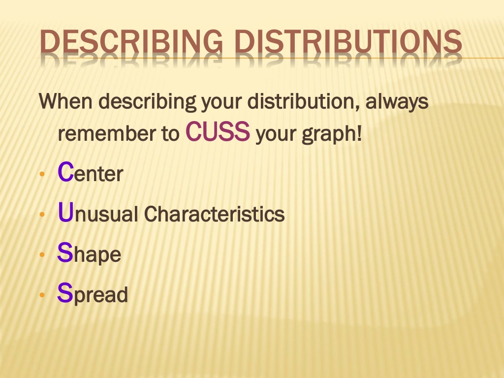
When describing a distribution, always remember to CUSS your graph! Focus on the Center, any Unusual Characteristics, the Shape, and the Spread of the data. This approach helps in effectively analyzing and communicating key aspects of the distribution.

caoimhe Follow

Uploaded on Jul 29, 2024 | 2 Views

Download Presentation

Please find below an Image/Link to download the presentation.

The content on the website is provided AS IS for your information and personal use only. It may not be sold, licensed, or shared on other websites without obtaining consent from the author. Download presentation by click this link. If you encounter any issues during the download, it is possible that the publisher has removed the file from their server.

E N D

Presentation Transcript

DESCRIBING DISTRIBUTIONS When describing your distribution, always When describing your distribution, always remember to remember to CUSS CUSS your graph! C Center enter U Unusual Characteristics nusual Characteristics S Shape hape S Spread pread your graph!

SHAPE 1. Does the histogram have a single hump or several separated humps? Unimodal Unimodal, Bimodal, or Multimodal , Bimodal, or Multimodal 2. Is the histogram symmetric or asymmetric? Symmetric Symmetric - - Uniform, Bell Shaped (Normal Distribution) Uniform, Bell Shaped (Normal Distribution) Asymmetric Asymmetric - - Skewed Right, Skewed Left Skewed Right, Skewed Left

MODES OF A HISTOGRAM Humps or peaks in a histogram are called Humps or peaks in a histogram are called modes modes. . A histogram with one main peak is dubbed A histogram with one main peak is dubbed unimodal unimodal. . A histograms with two peaks are A histograms with two peaks are bimodal. A histograms with three or more peaks are A histograms with three or more peaks are called called multimodal multimodal. . bimodal.

EXAMPLE OF BIMODAL DISTRIBUTION A bimodal histogram has two apparent peaks: A bimodal histogram has two apparent peaks:

AN EXAMPLE OF BIMODAL DISTRIBUTIONS AN EXAMPLE OF BIMODAL DISTRIBUTIONS The distribution of hours spent by U.S. The distribution of hours spent by U.S. adults watching football on Thanksgiving adults watching football on Thanksgiving Day Day Bimodal. Many people watch no football Bimodal. Many people watch no football (center is 0 hours), others watch most of (center is 0 hours), others watch most of one or more games (center is between 2 one or more games (center is between 2 and 3 hours). Probably only a few values and 3 hours). Probably only a few values over 5 hours. over 5 hours.

BIMODAL (CONT.) If there are multiple modes, try to If there are multiple modes, try to understand why. If you identify a reason understand why. If you identify a reason for the separate modes, it may be good to for the separate modes, it may be good to split the data into two groups. split the data into two groups.

EXAMPLE The dotplot to the right shows Kentucky Derby winning times. There are two clusters of points, one just below 160 seconds and the other at about 122 seconds. We found out that in 1896 the distance of the Derby race was changed from 1.5 miles to the current 1.25 miles, which explains the two clusters of winning times.

SYMMETRY If you can fold the histogram along a vertical line through the middle and have the edges match pretty closely, the histogram is symmetric.

SYMMETRY (CONT.) Two special symmetrical distributions Two special symmetrical distributions oBell Bell- -shaped shaped: has a center mound : has a center mound with two sloping tails. with two sloping tails. oUniform Uniform: refers to data in which : refers to data in which every class has equal or every class has equal or approximately equal frequency. approximately equal frequency.

UNIFORM DISTRIBUTIONS All the bars are approximately the same height (equal All the bars are approximately the same height (equal frequency). frequency). Doesn t appear to have any mode. Doesn t appear to have any mode. Symmetrical. Symmetrical.

AN EXAMPLE OF UNIFORM DISTRIBUTIONS The distribution of the last digit of phone The distribution of the last digit of phone numbers on our campus numbers on our campus uniform, symmetric, centered near 5. Roughly uniform, symmetric, centered near 5. Roughly equal counts for each digit 0 equal counts for each digit 0- -9. 9.

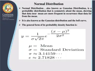
BELL SHAPED NORMAL DISTRIBUTION The normal distribution is symmetric and unimodal.

AN EXAMPLE OF NORMAL DISTRIBUTIONS The distribution of height of all adults There are very few people that are extremely tall or extremely short, but most tend to cluster around the average. Most things we measure tend to have a normal shape.

SKEWED (ASYMMETRICAL) The thinner ends of a distribution are called the The thinner ends of a distribution are called the tails If one tail stretches out farther than the other, the histogram If one tail stretches out farther than the other, the histogram is said to be is said to be skewed skewed to the side of the longer tail. to the side of the longer tail. In the figure below, the histogram on the left is said to be In the figure below, the histogram on the left is said to be left left- -skewed skewed, while the histogram on the right is said to be , while the histogram on the right is said to be right right- -skewed skewed. . tails. .

EXAMPLE The The distribtion distribtion of amount of winnings of all people playing a of amount of winnings of all people playing a particular state s lottery last week. particular state s lottery last week. Strongly skewed to the right, with almost everyone at $0, a few Strongly skewed to the right, with almost everyone at $0, a few small prizes, with the winner an outlier. small prizes, with the winner an outlier. The distribution of test scores in our AP Statistics class. The distribution of test scores in our AP Statistics class. Skewed to the left, with most of scores between 80 and 90 and Skewed to the left, with most of scores between 80 and 90 and a few in 50s. a few in 50s. Do not be confused about the Do not be confused about the skewness means there are lots of high scores and left skewed means there are lots of low means there are lots of high scores and left skewed means there are lots of low scores. scores. But it is just the opposite! But it is just the opposite! skewness. . Many people think that right skewed Many people think that right skewed

UNUSUAL CHARACTERISTICS Sometimes it s the unusual features that tell us something interesting or exciting about the data. You should always mention any stragglers, or outliers and the location of those outliers. Possible Causes: Possible Causes: Data Mistake Data Mistake Special nature of some observations Special nature of some observations Are there any gaps in the distribution? If so, what are the location of the gaps? 1. 1. 2. 2.

EXAMPLE The overall pattern is fairly symmetrical except for two states clearly not belonging to the main trend. Alaska has an unusually low (5%- 6%) percent of residents aged 65 or over, while Florida has an unusually high representation (18- 19%) of the elderly in their population. Two gaps are present between 6-8% and 16-18%. Alaska Florida

EXAMPLE The following histogram has outliers there are three cities in the leftmost bar A large gap in the distribution is typically a sign of an outlier. Gap Gap

UNUSUAL FEATURES If there are any clear outliers and you are reporting the mean and standard deviation, report them with the outliers present and with the outliers removed. The differences may be quite revealing. Note: The median and IQR are not likely to be affected by the outliers. So, report IQR and median if there are outliers.

Example Percent of people dying x = 4.2 With the outliers With the outliers x = 3.4 Without the outliers Without the outliers The mean is pulled to the right The median, on the other hand, a lot by the outliers is only slightly pulled to the right (from 3.4 to 4.2). by the outliers (from 3.4 to 3.6).

CENTER Tell (numerically) where the center of Tell (numerically) where the center of the data is. the data is. Mean average Median middle value when data is listed from low to high

MEAN MEAN Sum of data values divided by n Sum of data values divided by n parameter NOTE: NOTE: n n denotes the sample size Use Use to represent a population to represent a population mean mean Use to represent a sample mean Use to represent a sample mean x x n statistic x is the capital Greek letter sigma it means to sum the values that follow =

MEDIAN MEDIAN Median is the 50 Median is the 50th th percentile. percentile. Observations must be in numerical order. Observations must be in numerical order. A number is the A number is the ith the data is at or below the number. the data is at or below the number. ith percentile means that percentile means that i i% of % of Median is the middle single value if Median is the middle single value if n n is odd. is odd. n n denotes the sample size Median is the average of the middle two values if Median is the average of the middle two values if n n is even. is even.

EXAMPLE EXAMPLE Suppose we have sample of 6 customers that buy the following number of lollipops. The median is The median is 5 lollipops! The numbers are in order & n n is even so find the middle two observations. Now, average the 3rd (n/2) and the 4th (n/2 + 1) values. 5 5 2 3 4 6 8 12

EXAMPLE (CONT.) EXAMPLE (CONT.) To find the mean number of lollipops add the observations and divide by n n. 3 = x 4 . 5 8 833 + + + + + 2 6 12 6 2 3 4 6 8 12

RESISTENCE RESISTENCE What would happen to the median & mean if the 12 lollipops were 20? The median is . . .5 5 The mean is . . .7.17 7.17 + + + + + 2 3 4 6 8 20 6 What happened? 2 3 4 6 8 20

RESISTANCE (CONT.) RESISTANCE (CONT.) What would happen to the median & mean if the 20 lollipops were 50? The median is . . . The median is . . . 5 5 The mean is . . . The mean is . . .12.17 12.17 + + + + + 2 3 4 6 8 What happened? 50 6 2 3 4 6 8 50

RESISTANCE A Statistic is said to be resistant if outliers A Statistic is said to be resistant if outliers have only a small effect on it. have only a small effect on it. YES YES Is the median resistant? Is the median resistant? Is the mean resistant? Is the mean resistant? NO NO

MEAN, MEDIAN, AND HISTOGRAM MEAN, MEDIAN, AND HISTOGRAM Look at the following data set. Find the mean & median. 27 27 Mean Mean = Median Median = 27 27 Look at the placement of the mean and median in this roughly symmetrical distribution. Create a histogram (bin size is 2) 21 21 23 23 23 23 24 24 25 25 25 25 26 26 26 26 26 26 27 27 27 27 27 27 27 27 28 28 30 30 30 30 30 30 31 31 32 32 32 32

MEAN, MEDIAN, AND HISTOGRAM (CONT.) MEAN, MEDIAN, AND HISTOGRAM (CONT.) Look at the following data set. Find the mean & median. Mean Mean = Median Median = 25 25 28.176 28.176 Look at the placement of the mean and median in this right skewed distribution. Create a histogram (bin size is 8) 21 21 22 22 22 22 23 23 23 23 23 23 24 24 24 24 25 25 25 25 26 26 27 27 29 29 29 29 34 34 38 38 64 64

MEAN, MEDIAN, AND HISTOGRAM (CONT.) MEAN, MEDIAN, AND HISTOGRAM (CONT.) Look at the following data set. Find the mean & median. Mean Mean = Median Median = 58 58 54.588 54.588 Look at the placement of the mean and median in this left skewed distribution. Create a histogram (bin size is 8) 23 23 46 46 54 54 47 47 53 53 60 60 53 53 55 55 60 60 56 56 58 58 58 58 58 58 58 58 62 62 61 61 66 66

MEAN, MEDIAN, AND HISTOGRAM MEAN, MEDIAN, AND HISTOGRAM In a symmetrical distribution, the mean and In a symmetrical distribution, the mean and median are equal. median are equal. In a skewed distribution, the mean is pulled In a skewed distribution, the mean is pulled in the direction of the in the direction of the skewness In a In a symmetrical symmetrical distribution, you should distribution, you should report the report the mean mean because because mean resistant resistant against extreme values. against extreme values. In a In a skewed skewed distribution, the distribution, the median be reported as the measure of center be reported as the measure of center because because median median is is resistant resistant to extreme values in data set. values in data set. skewness. . mean is is NOT NOT median should should to extreme

Comparing the mean and the median The mean and the median are the same only if the distribution is symmetrical. The mean and the median are the same only if the distribution is symmetrical. The median is a measure of center that is resistant to skew and outliers. The mean is The median is a measure of center that is resistant to skew and outliers. The mean is not. not. Mean and median for a symmetric distribution Mean Mean Median Median Mean and median for skewed distributions Left skew Right skew Mean Mean Mean Mean Median Median Median Median

MEAN OR MEDIAN?

EXAMPLE Observed mean =2.28, median=3, mode=3.1 What is the shape of the distribution and why? Solution: Skewed Left Symmetr Symmetric ic Left Left- -Skewed Skewed Right Right- -Skewed Skewed Mean Mean Median Median Mode Mode Mean Mean = = Median Median = = Mode Mode Mode Mode Median Median Mean Mean

MEDIAN The median is the value with exactly half the data values below The median is the value with exactly half the data values below it and half above it. it and half above it.

MEAN The mean is located at the balancing point of the histogram. The mean is located at the balancing point of the histogram.

MATCH THE HISTOGRAMS TO THE SUMMARY STATISTICS

EXAMPLE For which of the distributions is the mean greater than the median? A

SPREAD Variation matters, and Statistics is about variation. Are the values of the distribution tightly clustered around the center or more spread out? Always report a measure of spread along with a measure of center when describing a distribution numerically.

MEASURES OF SPREAD The most commonly used measures of variability for sample data are the: range interquartile range variance or standard deviation

RANGE The range of a data set is the difference between the maximum and minimum values: range = max min The range is affected by outliers. The range does not utilize all the information in the data set only the largest and smallest values. A disadvantage of the range is that a single extreme value can make it very large, not representative of the overall data. Thus, it is not a very useful measure of spread or variation.

THE INTERQUARTILE RANGE A better way to describe the spread of a set of data might be to ignore the extremes and concentrate on the middle of the data. The interquartile range (IQR) lets us ignore extreme data values and concentrate on the middle of the data. To find the IQR, we first need to know what quartiles are

QUARTILES Quartiles Quartiles divide the data into four equal sections. divide the data into four equal sections. One quarter of the data lies below the lower quartile, One quarter of the data lies below the lower quartile, Q1, Q1, the 25 the 25th th percentile of ordered data or median of percentile of ordered data or median of lower half of ordered data lower half of ordered data Median (Q2) Median (Q2) is 50 is 50th th percentile of ordered data percentile of ordered data One quarter of the data lies above the upper quartile, One quarter of the data lies above the upper quartile, Q3, Q3, the 75 the 75th th percentile of ordered data or median of percentile of ordered data or median of upper half of ordered data upper half of ordered data

THE INTERQUARTILE RANGE IQR( IQR(Interquartile Interquartile Range) Q3 Q3 lower quartile Q1 lower quartile Q1 IQR is a measure of how spread out the is a measure of how spread out the middle 50% of values are. middle 50% of values are. Any point that falls outside the interval calculated by calculated by Q1 Q1- - 1.5(IQR) and Q3 + 1.5(IQR) and Q3 + 1.5(IQR) 1.5(IQR) is considered an is considered an outlier Range) = = upper quartile upper quartile IQR Any point that falls outside the interval outlier. .

Example 1 2 3 4 5 6 7 8 9 1 0.6 2 1.2 3 1.6 4 1.9 5 1.5 6 2.1 7 2.3 1 2.3 2 2.5 3 2.8 4 2.9 5 3.3 25% of data at or 25% of data at or below below Q Q1 1 Q Q1 1= first quartile = 2.2 = first quartile = 2.2 10 11 12 13 14 15 16 17 18 19 20 21 22 23 24 25 IQR = Q IQR = Q3 3 - - Q Q1 1 =4.35 =4.35 - - 2.2 =2.15 =2.15 2.2 M = M = median median = = 3.4 3.4 3.4 1 3.6 2 3.7 3 3.8 4 3.9 5 4.1 6 4.2 7 4.5 1 4.7 2 4.9 3 5.3 4 5.6 5 6.1 75% of data at or 75% of data at or below below Q Q3 3 Q Q3 3= third quartile = 4.35 = third quartile = 4.35

THE INTERQUARTILE RANGE The lower and upper quartiles are the 25 The lower and upper quartiles are the 25th th and 75 of the data, so of the data, so The IQR contains the middle 50% of the values of the The IQR contains the middle 50% of the values of the distribution, as shown in figure: distribution, as shown in figure: and 75th th percentiles percentiles

SKEWED DISTRIBUTION AND QUARTILES The sampling distribution of 143 bear weights in the The sampling distribution of 143 bear weights in the dotplot dotplot is skewed right. The median weight is about 155 is skewed right. The median weight is about 155 pounds. The middle 50% of the bear weights are between pounds. The middle 50% of the bear weights are between approximately 115 and 250 pounds. approximately 115 and 250 pounds.