Graph Machine Learning Overview: Traditional ML to Graph Neural Networks
Explore the evolution of Machine Learning in Graphs, from traditional ML tasks to advanced Graph Neural Networks (GNNs). Discover key concepts like feature engineering, tools like PyG, and types of ML tasks in graphs. Uncover insights into node-level, graph-level, and community-level predictions, and understand the traditional ML pipeline and feature designs. Dive into node classification and effective feature design for better model performance in graph-based machine learning.

Download Presentation

Please find below an Image/Link to download the presentation.
The content on the website is provided AS IS for your information and personal use only. It may not be sold, licensed, or shared on other websites without obtaining consent from the author. Download presentation by click this link. If you encounter any issues during the download, it is possible that the publisher has removed the file from their server.
E N D
Presentation Transcript
Online Social Networks and Media Graph ML I 1
Graph Machine Learning Outline Part I: Introduction, Traditional ML Part II: Graph Embeddings Part III: GNNs Part IV (if time permits): Knowledge Graphs Slides used based on: CS224W:Machine Learning withGraphs JureLeskovec,StanfordUniversity http://cs224w.stanford.edu 2
Part I: Types of ML Tasks Traditional ML Feature Engineering 3
Tools PyG (PyTorch Geometric): Theultimatelibrary for Graph Neural Networks We further recommend: GraphGym:Platformfor designingGraphNeural Networks. ModularizedGNN implementation, simple hyperparameter tuning, flexible user customization Other network analytics tools: SNAP.PY,NetworkX 4
Types of ML tasks in graphs Node level Graph-level prediction, Graph generation Community (subgraph) level Edge (link) level 6
Traditional ML Pipeline Designfeaturesfornodes/links/graphs Obtain featuresforall trainingdata ? ? ? Node features Link features B Graph features F A E D G C H 7
Traditional ML Pipeline Applythe model: Given a new node/link/graph, obtain its features and makea prediction Trainan ML model: Random forest SVM Neural network, etc. ?? ?1 ? ? ?? ?? 8
Node Level Tasks (example) ? ? ? ? Machine Learning ? Node classification 9
Feature Design Usingeffectivefeaturesovergraphs isthe key to achievinggood modelperformance. TraditionalML pipelineuses hand- designed features. We will overview traditional featuresfor: Node-level prediction Link-level prediction Graph-level prediction Forsimplicity, wefocuson undirectedgraphs. 10
Goal: Makepredictions for a set of objects Designchoices: Features:d-dimensional vectors Objects:Nodes,edges,sets of nodes, entiregraphs Objectivefunction: What task are we aiming to solve? 11
Node Level Features Goal: Characterizethe structureand position of a node in the network: Node degree Node centrality Node feature Clustering coefficient Graphlets B F A E D G C H 13
Node degree The degree ??of node ? is the number of edges (neighboringnodes)the nodehas. Treatsall neighboringnodesequally. ??= 2 ??= 1 B F ??= 4 A E D G C H ??= 3 14
Node centrality Nodedegree countsthe neighboringnodes withoutcapturingtheir importance. Nodecentrality ??takes the nodeimportance in a graphintoaccount Differentwaysto model importance: Engienvector centrality Eigenvector (Pagerank) centrality Betweenness centrality Closeness centrality and many others 15
Pagerank centrality A node ? is important if surrounded by important neighboring nodes ? ?(?). We model the centrality of node ? as the sum of the centrality of neighboring nodes: ?(?) ? ? = ?????????(?) ? ? 16
Betweness centrality A node is important if it lies on many shortest paths between other nodes. Example: ??= ??= ??= 0 ??= 3 (A-C-B,A-C-D,A-C-D-E) B A E D ??= 3 (A-C-D-E, B-D-E, C-D-E) C 17
Closeness centrality A node is important if it has small shortest path lengths to all other nodes. Example: ??= 1/(2+ 1 + 2 + 3) = 1/8 (A-C-B,A-C,A-C-D,A-C-D-E) B A E D ? = 1/(2 +1 + 1 + 1) = 1/5 ? (D-C-A, D-B, D-C, D-E) C 18
Clustering coefficient Measureshowconnectedthe neighboring nodesof ?are: #(node pairs among ??neighboringnodes) In our examples below the denominator is 6 (4 choose 2). Examples: ? ? ? ??= 0 ??= 0.5 ??= 1 19
Graphlets Observation:Clustering coefficientcountsthe #(triangles) in theego-network ? ? ? ? ??= 0.5 3 triangles (out of 6 node triplets) We can generalizethe abovebycounting #(pre-specified subgraphs),i.e., graphlets. 20
Graphlets Goal: Describenetworkstructurearound node? Graphlets aresmall subgraphs that describe the structure of node ? s network neighborhood B A E ? Analogy: C Degreecounts#(edges)thata nodetouches Clusteringcoefficientcounts#(triangles) thata nodetouches. GraphletDegreeVector(GDV): Graphlet-base featuresfor nodes GDV counts #(graphlets) that a node touches 21
Graphlets Def:Induced subgraph is another graph, formed from a subset of vertices and all the edges connecting the vertices in that subset. B A B B Induced subgraph: Not induced subgraph: E ? ? ? C C C 22
Graphlets Def:Graph Isomorphism Two graphs which contain the same number of nodes connected in the same way are said to be isomorphic. (one-to-one mapping of their nodes) Isomorphic Non-Isomorphic Node mapping: (e2,c2), (e1, c5), (e3,c4), (e5,c3), (e4,c1) The right graph has cycles of length 3 but the left graphdoesnot, so the graphs cannot be isomorphic. Source: Mathoverflow 23
Przulj et al.,Bioinformatics2004 Graphlets Graphlets:Rootedconnected induced non- isomorphicsubgraphs: All possible graphlets on up to 3 nodes Graphlet Degree Vector (GDV): Acount vectorofgraphletsrooted ata given node. 24
Graphlets All possible graphlets on up to 3 nodes Example: ? Graphlet instances of node u: ? ? ? ? Graphlets of node ?: ?,?,?,? [2,1,0,2] 25 28
Przulj et al.,Bioinformatics2004 Graphlets B A E ? C ? has graphlets: 0, 1, 2, 3, 5, 10, 11, Graphlet id(Root/ position of node ?) There are 73 different graphlets on up to 5 nodes 26
Graphlets Consideringgraphlets of size 2-5 nodesweget: Vector of 73 coordinates is a signature of a node that describes the topology of node's neighborhood Graphletdegreevectorprovidesa measureof a node s localnetworktopology: Comparing vectors of two nodes provides a more detailed measure of local topological similarity than node degrees or clustering coefficient B A E ? has graphlets: 0, 1, 2, 3, 5, 10, 11, ? C 27 C
Node Level Features Wehaveintroduceddifferentwaystoobtain node features. They can be categorizedas: Importance-based features: Node degree Differentnodecentrality measures Structure-based features: Node degree Clusteringcoefficient Graphlet countvector 28
Node Level Features Importance-basedfeatures:capture the importanceof a nodein a graph Node degree: Simply countsthe numberof neighboring nodes Node centrality: Models importanceof neighboring nodes in a graph Different modelingchoices: eigenvectorcentrality, betweennesscentrality, closenesscentrality Usefulfor predicting influentialnodesin a graph Example: predicting celebrity users in a social network 29
Node Level Features Structure-basedfeatures:Capture topological propertiesoflocalneighborhood aroundanode. Node degree: Countsthenumber ofneighboring nodes Clustering coefficient: Measures how connectedneighboring nodes are Graphlet degree vector: Counts theoccurrencesof differentgraphlets Usefulforpredictinga particularrole anode plays in a graph: Example: Predicting protein functionality in a protein-protein interaction network. 30
Node Level Tasks ? ? ? ? Machine Learning ? Node classification 31
Protein Folding Computationally predict the 3D structure of a protein based solely on its amino acid sequence: For each node predict its 3D coordinates 32 Imagecredit:DeepMind
Imagecredit: DeepMind Imagecredit: SingularityHub 33
Key idea: Spatial graph Nodes: Amino acids in a protein sequence Edges: Proximity between amino acids (residues) Spatial graph Imagecredit:DeepMind 34
Link Prediction Thetask is to predict newlinksbasedon the existinglinks. Two ways: (a) define a score for each pair of nodes, rank pairs, return top K ones, (b) build a classifier with input pair of nodes, output probability of existence ? B F A E D G C ? H 36
Link Prediction Thekey is to design features for apair of nodes. (for computing the score, as input to the classifier First, score ? B F A E D G C ? H 37
Link Prediction (1) Linksmissingat random: Missing/unknown, incomplete information Remove a random set of links and then aim to predict them 38
Link Prediction (2) Temporal Links Prediction Given ?[?0,? ] a graph defined by edges up to time ? , output a ranked list L of edges (not in ?[?0,? ]) that are predicted to appear in time ?[?1,?1] 0 0 0 ?[? ,? ] ?[?1,? ] 0 0 1 1 39
Score-based Link Prediction Methodology: For each pair of nodes (x,y) compute score c(x,y) Forexample, c(x,y) could be the# of commonneighbors of x and y Sort pairs (x,y) by the decreasing score c(x,y) Predict top n pairs as new links Evaluation: X n = |Enew|: # new edges thatappear during the testperiod [?1,? ] Taketopn elements of L and countcorrectedges 40
Link Level Features Distance-based feature Local neighborhoodoverlap Global neighborhoodoverlap Link feature B F A E D G C H 41
Distance-based Features Shortest-path distancebetweentwo nodes Example: B F ???= ???= ???= 2 ???= ???= 3 A E D G C H H However,thisdoesnotcapturethedegree of neighborhood overlap: Node pair (B, H) has 2 shared neighboring nodes, while pairs (B, E) and (A, B) only have 1 such node. 42
Local Neighborhood Overlap Features Local Neighborhood Features: Captures # neighboring nodes shared between two nodes Example: ?(?,?) Common neighbors: |? ?1 ?2| B ?? A Jaccard coefficient: E D |? ?1 ?2| |? ?1 ?2| C ?? F 43
Local Neighborhood Overlap Features Adamic-Adar index: 1 log(??) ? ? ?1 ?(?2) B ?? A E D C ?? F 44
Global Neighborhood Overlap Features Limitationof local neighborhood features: Metric is always zero if the two nodes do not have any neighbors in common. B ?? A ?? ??= ? |?? ??| = 0 E D C ?? F However, the two nodes maystill potentially connect in the future. Global neighborhoodoverlapmetrics resolve the limitation byconsideringthe entire graph. 45
Global Neighborhood Overlap Features Katz index: countsthe numberof walksof all lengths betweena given pairofnodes. How to compute #walksbetweentwo nodes? Usepowersof the adjacencymatrix! 46
Global Neighborhood Overlap Features Computing#walksbetweentwo nodes Recall: ???= 1 if ? ?(?) Let ?(?)= #walks of length ? between ? and ? ?? We will show ?(?)= ?? ?(?)= #walks of length 1 (direct neighborhood) between ? and ? = ??? ?? ?(?)= ??? ?? 4 3 2 1 47
Global Neighborhood Overlap Features How to compute Step 1: Compute #walks of length 1 between each of ? s neighbor and ? Step 2: Sum up these #walks across u s neighbors ? ?(?)= ? ?(?)= ? = ?? ? ?? ?? ?? ?? ?? ? ? ?? #walks of length 1 between Node 1 s neighbors and Node 2 ?(?)= ?2 Node 1 s neighbors 12 ?? Power of adjacency 48
Global Neighborhood Overlap Features Howto compute#walksbetween twonodes? Use adjacencymatrix powers ???specifies #walks of length 1 (direct neighborhood) between ? and ?. ??specifies #walks of length 2 (neighbor of ?? neighbor) between ? and ?. And, ?? specifies #walks of length ?. ?? 49
Global Neighborhood Overlap Features Katzindexbetween ?1and?2is calculatedas Sum over all walk lengths #walks of length ? between ?1and?2 0 < ? < 1: discount factor Katzindex matrixis computedin closed-form: = ???? by geometric series of matrices ?=0 5


")