Understanding Production Function and Laws of Returns in Economics

Production function in economics involves transforming inputs into outputs and understanding the relationship between input quantities and output under a given technology state. Concepts like Total Product, Average Product, and Marginal Product are essential in analyzing production efficiency. The Law of Variable Proportions, also known as the Law of Diminishing Marginal Returns, explains the behavior of production in the short run when varying one input while holding others constant.

Download Presentation

Please find below an Image/Link to download the presentation.
The content on the website is provided AS IS for your information and personal use only. It may not be sold, licensed, or shared on other websites without obtaining consent from the author. Download presentation by click this link. If you encounter any issues during the download, it is possible that the publisher has removed the file from their server.
E N D
Presentation Transcript
SEMESTER I Module III - SUPPLY AND PRODUCTION DECISIONS Production function: short run analysis with Law of Variable Proportions - Production function with two variable inputs - isoquants, ridge lines and least cost combination of inputs - Long run production function and Laws of Returns to Scale - expansion path - Economies and diseconomies of Scale and economies of scope
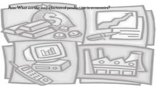
PRODUCTION FUNCTION Production: Production is the act of transforming inputs into outputs. In Economics, Production means creation of utility. Production function: It refers to the functional relationship between physical factor inputs and output of a firm per unit of time, under a given state of technology. It is basically engineering or technical relation showing how inputs are transformed or converted into output.
PRODUCTION FUNCTION Algebraically, ( ( ) ) Q = = f a, b, c...n, T Where, Q = Physical quantity of output f = functional relationship a, b, c n = quantities of various inputs = Constant Technology T
Concepts of Total Product, Average Product and Marginal Product Total Product (TP): It refers to the total amount of a commodity produced during a period of time, by using certain amount of inputs. ( ( ) ) TP = = f QVF Where, TP = Total Product QVF = Quantity of Variable Factor
Concepts Average Product (AP): It refers to total product per unit of a given variable factor. TP AP = = QVF Marginal Product (MP): It refers to the addition made to the total product by employing an additional unit of a factor. = = MP TP TP n n 1
Law of Variable Proportion or Law of Diminishing Marginal Returns This Law was developed by classical economist David Ricardo to explain the behaviour of agricultural output. It is also known as the law of diminishing returns. The law examines the behaviour of the production in the short run where the output is increased by increasing the units of variable factors, keeping other factors fixed.
Statement of the Law In the short run, as the amount of a variable factor increase, other things remaining constant, the output will increase more than proportionately in the initial stage, then it may increase in the same proportion and lastly it will increase less than proportionately.
Production Schedule Units of Variable factor 1 2 3 4 5 6 7 Total Product (TP) 2 10 30 40 45 48 49 Average Product (AP) 2 5 10 10 9 8 7 Marginal Product (MP) 2 8 20 10 5 3 1 Stages of Production Stage I Stage II 8 48 6 -1 Stage III
Explanation of the table Stage 1: Initially the TP increases at an increasing rate along with that the AP and the MP also rise. This is the stage of increasing returns. When the TP is maximum, the AP = MP at 4th unit i.e. the same 10. Stage 2: After a certain point, the MP begins to diminish. Hence the TP increases at a diminishing rate. When the MP becomes zero, the TP is the maximum i.e. 49 at 7th unit. Stage III: When the MP becomes negative at 8th unit, the TP begins to decline in the same proportion. The AP also decreases but remains positive.
Law of Variable Proportions 60 TP 50 40 30 TP, AP, MP 20 AP 10 0 1 2 3 4 5 6 7 8 MP -10 Units of Variable Factor MP TP AP
Explanation of the diagram Reasons for increasing, diminishing and negative returns: Increasing Returns: In the initial stage of production the returns to variable factors increase due to the large quantity of fixed factor. The fixed factor is effectively used, as additional units of variable factors are employed. In agriculture, land which is the fixed factor is cultivated better. For instance, labour becomes efficient due to division of labour and specialisation.
Explanation of the diagram Diminishing Returns: Increasing returns come to an end when the maximum point is reach. The fixed factor is not enough for the efficient use of extra units of variable factor. Every extra unit of variable factor produce less output because the extra units of variable factor have less and less fixed factor to work with. Diminishing returns are the result of congestion. Negative Returns: The negative returns are the result of too many units of variable factor working on fixed factor. In our example, there are too many labourers having insufficient work thus creating disturbances to each other.
Types of production Function Short run: It refers to the period of time over which one (or more) factor(s) of production is (are) fixed. In the real commercial world, land and capital (such as plant and equipment) are usually treated as fixed factors. In a simple production process with only two factors i.e. capital as the fixed factor and labour as the variable factor. ( ( ) ) = = Q f L C ,
Types of production Function Long run: It is defined as that period over which all factors of production can be changed, with the given state of technology. In the long run all factors are variable. The size of the plant and its scale of production can be fully increased or decreased. ( ( ) ) = = Q f L C ,
Types of Isoquant Isoquant or Equal Product Curve: It represents all those combinations of two factors inputs (Labour and Capital) which produce the same level of output. Types of Isoquant: 1. Linear Isoquant 2. Right Angled Isoquant 3. Kinked Isoquant 4. Smooth Convex Isoquant
1. Linear Isoquant In the above diagram, at point A on the isoquant the level of output can be produced with alone (without labour). Similarly, at point B the level of output can be produced with alone (without capital). This is unrealistic, because output is function of both labour and capital. Y A capital Capital Isoquant labour B X 0 Labour
2. Right Angled Isoquant Y In this case, the isoquant would be right angle. This type assumes complements of factors of production i.e. labour and capital must be used in fixed proportion shown by Point C. This isoquant is also known as Leontief isoquant after Leontief, who developed the input-output model. Isoquant perfect Capital C Wassily X 0 Labour
3. Kinked Isoquant In the above diagram, A1, A2, A3 and A4 show the production process and Q is the kinked isoquant. Here, the substitution of factors is possible only at the kinks, i.e. at point A, B, C and D. A Y 1 A 2 A 3 Capital A 4 A BCD Isoquant X 0 Labour
4. Smooth Convex Isoquant Y This type assumes continuous substitution of labour and capital. Capital Isoquant X 0 Labour
ISO-QUANT Isoquant or Equal Product Curve: It represents all those combinations of two factors inputs (Labour and Capital) which produce the same level of output. Properties of Isoquant: 1. Isoquants have negative slope 2. Isoquants are convex to origin 3. Isoquants do not intersect 4. Isoquants do not touch either axis
1. Isoquants have negative slope Y Capital a K 1 b K 2 = = IQ Units 100 X 0 L L Labour 1 2
2. Isoquants are convex to origin Y K = = MRTS Di min ishing L LK Capital a K 1 b K K c 2 3 d K 4 = = IQ Units 100 X 0 L L L L Labour 3 1 2 4
3. Isoquants do not intersect Y Capital a b 2= = IQ Units 200 1= = IQ Units 100 c X 0 Labour
4. Isoquants do not touch either axis Y Capital a IQ 2 IQ 1 b X 0 Labour
Ridge lines Meaning: The ridge lines are the locus of points of isoquants where the marginal products (MP) of factors are zero. The upper ridge line implies zero MP of capital and the lower ridge line implies zero MP of labour. the curves IQ1, IQ2 and IQ3 are the oval shaped isoquants. The curves OA and OB are the ridge lines on the oval shaped isoquants. The points C, D, E, and F, G, H between the ridge lines are economically feasible units of capital and labour which can be employed to produce 100, 200 and 300 units of output.
In the diagram, OT units of labour and ST units of capital can produce 100 units of the output. The same output can be produced by using the same quantity of labour OT and less quantity of capital CT. Y Ridge Line Capital IQ3 ( 300 ) A S E B D IQ2 ( 200 ) C H IQ1 100 ( ) G F X O T Labour
Producers Equilibrium or Least Cost Factor Combination An isoquant or equal product curve indicates the various factor combinations which can yield various levels of output. A set of iso-cost line indicates the various levels of total cost or outlay given the prices of two factors. Thus, least cost factor combination refers to an optimum combination which yields maximum output at minimum cost.
Producers Equilibrium or Least Cost Factor Combination Assumptions: 1. There are two factors, labour and capital. 2. All units of labour and capital are homogeneous. 3. The factors prices are given and constant. 4. The cost outlay (total cost) is given. 5. There is perfect competition in factor market. 6. A firm should be rational i.e. tries to maximum satisfaction. Given these assumptions, producer s equilibrium point is that where the isoquant is tangent to an iso-cost line.
Iso-cost Line Isocost line is graphical representations of various combinations of the two factors that can be used by a firm from a given total cost or factor prices. Y A Capital P OA L = = = = Slope of isocost line OB P K Isocost line B X 0 Labour
A rational firm faces two choices of optimal combination of factors: 1. Minimisation of cost subject to given level of output. 2. Maximisation of output subject to given cost. 1. Minimisation of cost subject to given level of output: The firm maximises its profits by minimising its cost, given the output. A produces will try to produce given level of output with least cost combination of factors. This is explained in above diagram.
1. Minimisation of cost subject to given level of output Y Capital A P 4 A 3 Q A 2 A 1 E K C R S 1= = IQ Units 100 X 0 B B B B L 3 4 1 2 Labour
2. Maximisation of output subject to given total cost Y Capital H A 1 L V M K 4= = IQ Units 400 3= = IQ Units 300 N 2= = IQ Units 200 K 1= = IQ Units 100 X 0 L B Labour 1
LAW OF RETURNS TO SCALE It refers to the long run analysis of the laws of production. In the long run output can be increased by changing all factors. Statement of the law: Other things being equal, in the long run, as the firm increases the quantities of all factors employed the output may rise initially at a more rapid rate than the rate of increase in inputs, then output may increase in the same proportion of inputs and finally, output increases less than proportionately.
1. Increasing Returns to Scale Y E Capital c K 3 b K a 2 K 3= = IQ Units 300 1 2= = IQ Units 200 1= = IQ Units 100 X 0 L L L Labour 1 3 2
2. Constant Returns to Scale Y E Capital c K 3 b K 2 3= = IQ Units 300 a K 1 2= = IQ Units 200 1= = IQ Units 100 X 0 L L L Labour 1 3 2
3. Decreasing Returns to Scale Y E Capital c K 3 b K 3= = IQ Units 2 300 a K 1 2= = IQ Units 200 1= = IQ Units 100 X 0 L L L Labour 1 3 2
Economies of Scale In Monetary Sector a) Output b) Cost of production c) Investment d) Prices e) Business Environment a) Surplus budget b) Credit policy c) Money markets d) Interests a) Middle class b) Trade unions c) Wages d)Consumption expenditure
Economies of Scale Internal Economies of Scale External Economies of Scale 1. Managerial economies 2. Technical economies 3. Economies of by product 4. Economies of supervision 5. Economies of cost 6. Economies of integration 7. Risk bearing economies 8. Economics of specialization 1. Economies of large scale production 2. Economies of technical know-how 3. Economies of marketing 4. Economies of finance 5. Economies of environment 6. Economies of Information Services