Understanding Production Decision Making in Livestock Economics and Marketing

Dr. Puspendra Kumar Singh discusses the Theory of Production in livestock economics, covering topics such as how much to produce, how to produce, and what to produce. He explains the factors affecting production decisions, including input-output relationships and different types of production functions.
- Livestock Economics
- Production Decision
- Marketing Strategies
- Factor-Product Relationship
- Livestock Management

Download Presentation

Please find below an Image/Link to download the presentation.
The content on the website is provided AS IS for your information and personal use only. It may not be sold, licensed, or shared on other websites without obtaining consent from the author. Download presentation by click this link. If you encounter any issues during the download, it is possible that the publisher has removed the file from their server.
E N D
Presentation Transcript
UNIT-6 (LIVESTOCK ECONOMICS AND MARKETING) Lecture- 10thday Speaker :- Dr. Puspendra Kumar Singh Asstt. Professor Department of Veterinary & Animal Husbandry Extension Education, BVC
Topics covered Theory of Production.
Production Production : creation of utility Utility : Ability / Power of a good or service to satisfy human want. Input------------------------------------ Output. Production process 1. Creation of want satisfying Goods and services. 2. Creation of exchange value Basic Problems in Production involve production decision:- 1. How much to produce. 2. How to produce. 3. What to produce.
How much to produce It is problem related to the optimal level of resources use or the level of resource which maximize the profit. This problem has to be analyzed in the context of Factor - Product Relationship. Relationship between inputs and output of an enterprise has been called Production function. There are two kind of factor- product relationship in production function: 1. Proportionality relationship: Some inputs are fixed while quantities of other inputs vary. Corresponds to short run production, where there is not possible to increase all resources. Law of variable proportion or law of diminishing return. 2. Scale relationship: All the inputs are variable, none are fixed. Long run production, which allow all the resources to increase with increase in production. Law of return to scale.
How to produce It is problem related to what method and combination of resources to use. We have to assess least cost combination of different resources. Since, we are dealing with optimum (least cost) combination of resources that maximize the profit. This problem has to be analyzed in the context of least cost combination of resources. What to produce It is problem related to problem of enterprise selection or what product to be produced and in what combination when a fixed set of inputs is available. Producer has to make decision about profit maximizing combination of different product. This problem has to be analyzed in the context of product product relationship and govern by the principle of optimum combination of outputs.
There can be three types of input-output relationships in the production of a commodity, where one input is varied and the quantities of all other inputs are fixed. The relationship that takes place between single variable input and the consequent output pertains to either one or a combination of the following relationships: i. Constant marginal rate of returns (Constant productivity) ii. Increasing marginal rate of returns (Increasing productivity) iii. Decreasing marginal rate of returns (Decreasing productivity) 1. Constant marginal rate of returns In constant returns, each additional unit of variable input produces an equal amount of additional product. i.e., The amount of product increases by the same magnitude for each additional unit of input.
However, this is not a very common relationship in Animal Husbandry but may be possible in other industries. (Value of each Unit of input Rs. 1500) No. of units of Input (X) Total output (Y) Y X MP ( Y/ X) Average Variable cost = Unit variable cost /AP 0 - - - 10 500 500 10 50 1500/50 = 300 20 1000 500 10 50 1500/50 = 300 30 1500 500 10 50 1500/50 =300 40 2000 500 10 50 1500/50 =300 50 2500 500 10 50 1500/50 =300 The table show that every equal increase in the input results in a constant increase in the output and hence, the given production function is known as a constant marginal returns function giving a straight line production curve (TP curve) which is having the same slope throughout its entire range.
Y X-----------------
Increasing marginal rate of returns In this case, every additional or marginal unit of input adds more and more to the total product than the previous unit. i.e., addition to total product is at an increasing rate. In actual practice, the cases of purely increasing returns are rarely available.(Value of one unit of input Rs 500). No. of units of Input (X) 10 20 30 40 50 Total output (Y) Average Variable cost =Unit variable cost /AP X Y MP ( Y/ X) 100 - - - 500/10 =50 110 10 10 1 500/5.5 = 90.90 190 10 90 9 500/6.33 =78.99 300 10 110 11 500/7.5 = 66.67 450 10 150 15 500/9.0 = 55.56
Decreasing marginal rate of returns THE Addition of each successive unit of the variable factor to the fixed factors in the production process, adds less to the total output than the previous unit. No. of units of Input (X) 10 20 30 40 50 Total output (Y) X Y MP ( Y/ X) 100 - - - 150 10 50 5 190 10 40 4 220 10 30 3 240 10 200 2
Y X
Law of Variable Proportion or Law of Diminishing Return If the quantity of one productive service is increased by equal increments, with the quantity of other resource services held constant, the increments to total product may increase at first but will decrease after a certain point E.O.Heady An increase in capital and labour applied in cultivation of land causes in general, less than proportionate increase in the amount of product raised, unless it happens to coincide with an improvement in the arts of agriculture Marshall.
As the amount of variable resource used in production of a product is increased, the output of the product will at first increase at an increasing rate, then increase at a decreasing rate and finally a point will be reached, where further application of the variable resource will result in a decline in the total output of production. In short, marginal product of variable input will first increase, then decrease and finally become negative
Short Run and Long Run Short run refers to a period of time in which the supply of certain inputs (e.g. plant, building and machines, etc.) is fixed or inelastic. In short run, therefore, production of a commodity can be increased by increasing the use of variable inputs, like labour and raw materials. They do not refer to any fixed time period. While in some industries short term may be a matter of a few weeks or a few months, in some others (e.g., electric and power industry), it may mean three or more years. Long run refers to a period of time in which the supply of all the inputs is elastic, but not enough to permit a change in technology. In long run, the availability of even fixed factor increases. Therefore, in long run, production of commodity can be increased by employing more of both, variable and fixed, inputs. In the very long run, the production function also changes. The technological advances mean that a larger output can be created with a given quantity of inputs.
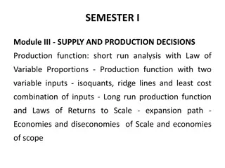
Short run production with one variable input Laws of returns state the relationship between the variable input and the output in the short term. By definition, certain factors of production (viz., land and capital equipment such as plant and machinery) are available in short supply during the short run. Such factors are known as fixed factors. On the other hand, the factors which are available in unlimited supply even during the short periods are known as variable factors. In short run, therefore, the firms can employ a limited or fixed quantity of fixed factors and an unlimited quantity of the variable factor. In other words, firms can employ in the short run, varying quantities of variable inputs against a given quantity of fixed factors. This kind of change in input combination leads to variation in factor proportions. The laws which bring out the relationship between varying factor proportions and output are therefore known as the Law of Variable Proportions, or what is more popularly known as the Law of Diminishing Returns.
Long term production with two variable inputs We shall now discuss the relationships between inputs and output under the condition that both the inputs, capital and labour, are variable factors. This is a long run phenomenon. In the long run, supply of both the inputs is supposed to be elastic and firms can hire larger quantities of both labour and capital. With large employment of capital and labour, the scale of production changes. The technological relationship between changing scale of inputs and output is explained through the production function and isoquant curves techniques. Production rules for the short run There are three rules for making production decisions in the short run. They are Expected selling price is greater than minimum ATC (or TR greater than TC). A profit can be made and is maximized by producing where MR = MC. Expected selling price is less than minimum ATC but greater than minimum AVC (or TR is greater than TVC but less than TC). A loss cannot be avoided but will be minimized by producing at the output level where MR=MC. The loss will be somewhere between zero and the total fixed cost. Expected selling price is less than minimum AVC (or TR less than TVC). A loss can not be avoided but is minimized by not producing. The loss will be equal to TFC. Application of these rules is as follows. With a selling price equal to MR1, the intersection of MR and MC is well above ATC, and a profit is being made.
")