Overview of Mechanics and Continuum Mechanics
Mechanics explores the motion of matter and forces influencing it, covering topics such as Elasticity, Plasticity, and Viscoelasticity. Continuum Mechanics delves into the mechanics of bodies, focusing on continuity, homogeneity, and isotropy. Understanding external forces, stresses, and elasticity are crucial in these fields as they shape the behavior of materials and structures.

Download Presentation

Please find below an Image/Link to download the presentation.
The content on the website is provided AS IS for your information and personal use only. It may not be sold, licensed, or shared on other websites without obtaining consent from the author. Download presentation by click this link. If you encounter any issues during the download, it is possible that the publisher has removed the file from their server.
E N D
Presentation Transcript
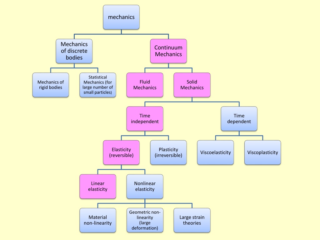
mechanics Mechanics of discrete bodies Continuum Mechanics Statistical Mechanics (for large number of small particles) Fluid Solid Mechanics of rigid bodies Mechanics Mechanics Time Time independent dependent Elasticity (reversible) Plasticity (irreversible) Viscoelasticity Viscoplasticity Linear elasticity Nonlinear elasticity Geometric non- linearity (large deformation) Material non-linearity Large strain theories
Continuum Mechanics References Continuum Mechanics for Engineering by G. Thomas Mase and George E. Mase. Advance Solid Mechanics by P.R. Lancaster and D. Mitchell. Advance Strength and Applied Elasticity by A.C. Ugural and S.K. Fenster. 1.Definitions Mechanics: The study of the motion of matter and the forces that cause such motion. Based on concepts of time, space, force, energy, and matter. Applications to point mass, solid bodies familiar from introductory physics. Continuum Mechanics: Mechanics of parts of bodies . Continuum: define values of fields (e.g., density) as functions of position, i.e., at points. M p n 0 Example: density , = ( ) lim n V1 V V n V2 P Vi : Sequence of volumes converging on (p). V3 Mi : Mass enclosed by Vi
Continuity: Completely fills space (no pores or void) and has properties describable by continuous functions. Homogeneity: Identical properties at all points (scale dependent). Isotropy: Properties same in all directions. 2. External Forces: There are two types of forces: a) Surface forces: Forces distributed over the surface of the body. (atmospheric pressure, hydraulic pressure) b) Body Forces: Forces distributed over the volume of the body. (gravitational forces, centrifugal forces, inertia forces) Note: A body responds to the application of external forces by deforming and by developing internal forces. Newton s 2nd low: F=ma, or F-ma=0 For this course, usually a=0 the governing equation is F=0. Applies not just to particles, entire bodies, but to regions with in bodies. Free-body diagram: cut open body (thought experiment), examine forces of interaction between surfaces.
Elasticity:The material returns to its original (unloaded) shape upon the removal of applied forces. stress stress loading loading unloading unloading strain strain Linear elastic material Nonlinear elastic material The graphs follow the same line whether loading or unloading
3. Stresses (Tractions) Stress is a measure of the internal forces per unit area within a body. S1 Fs1 y y Fn P A o x S2 o x Fs2 z z F is the force acting on an element of area A. n, s1 , s2 constitute a set of orthogonal axes, origin placed at the point P, with n normal and s1 , s2 tangent to A. Decomposition of F into components parallel to . n, s1 , and s2 then the normal stress n and the shear stresses are given by:
F = lim n n A 0 A F = 1 lim s 1 s A 0 A F = 2 lim s 2 s A 0 A A set of stresses on an infinite number of planes passing through a point forms the state of the stress at point.
4. Tensors Most physical quantities that are important in continuum mechanics like temperature, force, and stress can be represented by a tensor. Temperature can be specified by stating a single numerical value called a scalar and is called a zeroth-order tensor. A force, however, must be specified by stating both a magnitude and direction. It is an example of a first-order tensor. Specifying a stress is even more complicated and requires stating a magnitude and two directions the direction of a force vector and the direction of the normal vector to the plane on which the force acts. Stresses are represented by second- order tensors. 4.1. Stress Tensor Representing a force in three dimensions requires three numbers, each referenced to a coordinate axis. Representing the state of stress in three dimensions requires nine numbers, each referenced to a coordinate axis and a plane perpendicular to the coordinate axes.
To determining traction vectors on arbitrary surfaces. Consider two surfaces S1 and S2 at point Q. Tractions at a point depend on the orientation of the surface How to determine T, given n
yy yx yz xy xx zy zx xz y zz For special cases n along axes x z In vector notation, the tractions on the faces of the cube are written: = , , T x xx xy xz = , , T y yx yy yz = , , T z zx zy zz
In matrix notation, the tractions are written: T x xx xy xz = T y yx yy yz T z zx zy zz This matrix is generally referred to as the stress tensor. It s the complete representation of stress at a point
4.2. The Cauchy Tetrahedron and Traction on Arbitrary Planes Often, it is important to determine the state of stress on an arbitrarily oriented plane. y Tn Ty T B p Tx zz Ts Tz xz zx xx zy A o x xy yz yx C Stress acting on plane ABC yy z
Considering op to be normal to ABC, its line of orientation with respect to the x-y-z coordinate system is defined by the three direction cosines shown below p p x y o o A B op= op= = cos l = cos m oA oB p z o C op= = cos n oC Let the total stress (traction) acting on ABC is T, this would produce stress component Tx , Ty , Tz as shown in the above figure. Where (1) x T T + = + 2 2 2 2 T T y z
If stress components perpendicular and parallel to ABC plane are of greater concern, we find = + 2 2 2 (2) T T T n s Now, taking a force balance in the x-direction Fx =0 , gives (3a) xx x l T + = + m n yx zx And from Fy =0 and Fz =0 , we get T (3b) xy y l + = + m n yy zy (3c) xz z l T + = + m n yz zz Vector analysis gives, (4) x n lT T = ( x s T T + = + + mT nT y z ) + 2 2 2 2 T T T y z n (5)
Also Tn can be determined from the direction cosines and the known stresses as follows: ( ) = + + + + + 2 2 2 2 T l m n lm mn nl n xx yy zz yx yz zx In essence, no shear component acts on ABC and the direction cosines defining the line from the origin, o, that is now normal to ABC, however l, m, and n can still be used with this in mind: = = = , , T lT T mT T nT x y z The above relationships, it substituted into eq.(3), produce the following ( ) + + = 0 l T m n xx yx zx ( ) + + = 0 l m T n (6) xy yy zy ( ) + + = 0 l m n T xz yz xx
These three homogeneous equations gives real roots other than zero only, if the determinant is zero. Setting the determinant to zero and expanding gives a cubic equation chose three roots are the principal stresses (i.e. the stresses on plane of zero shear stress). Denoting the stress T as Tp gives: = 3 p 2 p 0 T I T I T I (7) 1 2 3 p Where I1 , I2 , and I3 are called the Invariants, and they given by ( xx I + = 1 ) + (9a) yy zz ( ) = + + 2 2 2 I (9b) 2 xy yz zx xx yy yy zz zz xx ( ) = + 2 yz 2 zx 2 xy 2 I (9c) 3 xx yy zz xy yz zx xx yy zz
4.3. Different Notations 1. A general equation for explicit expressions is given by: = 1 j 3 = T n i ji j 2. Summation notation is a way of writing summations without the summation sign . To use it, simply drop the and sum over repeated indices. The equation in summation notation is given by: n T = i ji j 3. The equation in matrix form is given by: T n 1 11 21 31 1 = T n 2 12 22 32 2 T n 3 13 23 33 3
4.4. Feature of the Stress Tensor The stress tensor is a symmetric tensor, meaning that ij= ji . As a result, the entire tensor may be specified with only six numbers instead of nine. y or 21 yx or dy 12 xy dx x Consider the moment M acting on an element with sides dx and dy dx dy M = 2 dy 2 2 = 0 dx z xy yx 2 = xy yx = = ; A similar argument shows Shears are always conjugate . yz zy xz zx
Example (1): An applied stress state is described by 20 3 8 = 3 15 5 ij 8 5 10 (Note: all stresses are indicated as positive) Determine the magnitude of the total state of stress , T, and its normal component, Tn , acting on plane whose direction cosines are given by (l=0.707, m=0.643, and n=0.296).
Example (2): A given stress state is expressed as 4 2 3 = 2 6 1 ij 3 1 5 The unit of each stress are in MPa and all stresses are denoted as positive. Find the magnitudes of the principle stresses and the direction cosines defining the line of action the largest principle stress with respect to the original x-y-z coordinate system.
4.5. Quantities in Different Coordinate Systems To provide a systematic approach to the transformation of stress from one coordinate system to another. Consider the following situation, where forces Fx , Fy , and Fz act along the x, y, z reference axes. y y Fy Fy x x Fx x z o x x o Fx Fz Fz z z Transformation of forces from one coordinate system to another
Now, assume y is the same as y such that the new x and z axes are in the same plane as x and z. the force component Fx is composed of the projections of Fx and Fzon the x axis, thus. = + cos cos F F F x x x x z x z = = , cos cos , Since l and n then x x x z = + F l F n F x x z In the general situation, the force Fy would also contribute to Fx , as follow: = + + F l F m F n F (10) x x y z Similar relationships could be developed for Fy and Fz using the proper set of direction cosines for each transformation. = = = = , , , , , , , cos F l F j x y z i x y z l i ij j ij ij
For the transformation of matrix quantities such as stress, first consider the following situation, where the uniaxial tensile stress yy is imposed. y y yy y y y y Ay yy Ay y Ay y x x x x x z yy Uniaxial stress transformation to an x , y , z system
= F A The force in the y-direction is y yy y Thus is the component of Fy acting along y y y y F F cos = the y -axis. The area Ay which is normal to y is : = cos A A y y y y cos F F y y y y = = Therefore, y y cos A A y y y y = 2 cos y y y yy y
For the fully generalised case, this type of transformation is expressed as: = im l l ij jn mn With m, n iterated over x, y, z and i, j iterated over x , y , z . Thus, the complete expression for x x becomes: + = + + l l l + l l l x x x x l x x l xx x y l x y l yy x z x z zz + l l x y y x x xy x x z yz x z x x zx + + + l l l l l l y x y x (11) x x yx x z x zy x x z xz = = = , , . Where etc xy xy yz yz zx zx
Rearrange the terms, gives ( ) = + + + + + 2 2 2 2 l l l l l l l l l x y x y y x x x x x y x z z x x xy x x z yz x z x zx Knowing that , we get l l l y x x x = = , = , m l n x z ( ) = + + + + + 2 2 2 2 l m n l m m n l n (12) x x y z xy yz zx Similarly from eq.(11) by appropriate interchange of subscripts, equivalent expressions for , etc. , , y z x y
4.6. Equilibrium Equations (Naviers Equation) Consider a small parallelepiped with sides of lengths dx, dy, and dz. y y + dy y yz + dy y yz yx + y dy yx y dx dz dy z + x dx x x Y x X x Z xy + dx xy x zy + y dz + xz dx zy z xz x z + zx dz + z dz zx z z z
Consider the equilibrium of forces in the x-direction + + . . . . . . . . x X dx dy dz dy dz dx dy dz dz dx x x yx x yx + + + + = . . . . 0 zx dy dx dz dy dx dz dy dx yx zx zx y z Where X is the x component of the body forces per unit volume. Canceling (dx.dy.dz) xy + + + = 0 x xz X (13) x y z Similarly yx y yz + + + = 0 Y (14) x y z
zy + + + = 0 zx z Z (15) x y z Here Y and Z are the y and z components of the body forces per unit volume. Equations 13 to 15 are Navier s equations of equilibrium for an elastic solid.


 and")

")


: An applied stress state is described by")
: A given stress state is expressed as")


")