Exploring Quantum Mechanics: Illusion or Reality?

Q
U
A
N
T
U
M
M
E
C
H
A
N
I
C
S
-
I
l
l
u
s
i
o
n
o
r
R
e
a
l
i
t
y
?
Prof. D. M. Parshuramkar
Dept. of Physics
N. H. College, Bramhapuri
1
.
C
l
a
s
s
i
c
a
l
M
e
c
h
a
n
i
c
s
•
Do the electrons in atoms and molecules obey
Newton’s classical laws of motion?
•
We shall see that the answer to this question is “No”.
•
This has led to the development of
Quantum
Mechanics
– we will contrast classical and quantum
mechanics.
1
.
1
F
e
a
t
u
r
e
s
o
f
C
l
a
s
s
i
c
a
l
M
e
c
h
a
n
i
c
s
(
C
M
)
1)
CM predicts a precise trajectory for a particle.
•
T
h
e
e
x
a
c
t
p
o
s
i
t
i
o
n
(
r
)
a
n
d
v
e
l
o
c
i
t
y
(
v
)
(
a
n
d
h
e
n
c
e
t
h
e
m
o
m
e
n
t
u
m
p
=
m
v
)
o
f
a
p
a
r
t
i
c
l
e
(
m
a
s
s
=
m
)
c
a
n
b
e
k
n
o
w
n
s
i
m
u
l
t
a
n
e
o
u
s
l
y
a
t
e
a
c
h
p
o
i
n
t
i
n
t
i
m
e
.
•
N
o
t
e
:
p
o
s
i
t
i
o
n
(
r
)
,
v
e
l
o
c
i
t
y
(
v
)
a
n
d
m
o
m
e
n
t
u
m
(
p
)
a
r
e
v
e
c
t
o
r
s
,
h
a
v
i
n
g
m
a
g
n
i
t
u
d
e
a
n
d
d
i
r
e
c
t
i
o
n
v
=
(
v
x
,
v
y
,
v
z
)
.
2)
Any type of motion
(translation, vibration, rotation)
can have any
value of energy associated with it
– i.e. there is a
continuum
of energy states.
3)
Particles and waves are distinguishable phenomena, with different,
characteristic properties and behaviour.
Property
Behaviour
mass
momentum
Particles
position
collisions
velocity
Waves
wavelength
diffraction
frequency
interference
1
.
2
R
e
v
i
s
i
o
n
o
f
S
o
m
e
R
e
l
e
v
a
n
t
E
q
u
a
t
i
o
n
s
i
n
C
M
Total energy of particle:
E
=
Kinetic Energy (KE)
+
Potential Energy (PE)
E =
½mv
2
+
V
E
=
p
2
/
2
m
+
V
(
p
=
m
v
)
N
o
t
e
:
s
t
r
i
c
t
l
y
E
,
T
,
V
(
a
n
d
r
,
v
,
p
)
a
r
e
a
l
l
d
e
f
i
n
e
d
a
t
a
p
a
r
t
i
c
u
l
a
r
t
i
m
e
(
t
)
–
E
(
t
)
e
t
c
.
.
T
-
d
e
p
e
n
d
s
o
n
v
V
-
d
e
p
e
n
d
s
o
n
r
V depends on the system
e.g. positional, electrostatic PE
•
Consider a 1-dimensional system (straight line translational
motion of a particle under the influence of a potential acting
parallel to the direction of motion):
•
Define:
position
r
= x
velocity
v
= dx/dt
momentum
p
= mv = m(dx/dt)
PE
V
force
F
=
(dV/dx)
•
Newton’s 2
nd
Law of Motion
F
= m
a
= m(dv/dt) = m(d
2
x/dt
2
)
•
Therefore, if we know the forces acting on a particle we can
solve a
differential equation
to determine it’s
trajectory
{x(t),p(t)}.
1
.
3
E
x
a
m
p
l
e
–
T
h
e
1
-
D
i
m
e
n
s
i
o
n
a
l
H
a
r
m
o
n
i
c
O
s
c
i
l
l
a
t
o
r
•
The particle experiences a
restoring force
(
F
) proportional to its
displacement (
x
) from its equilibrium position (x=0).
•
Hooke’s Law
F =
k
x
k
is the
stiffness of the spring
(or
stretching force constant
of the
bond if considering molecular vibrations)
•
Substituting F into Newton’s 2
nd
Law we get:
m(d
2
x/dt
2
) =
k
x
a (second order) differential
equation
NB
– assuming no friction or
other forces act on the particle
(except F).
k
Solution:
position
x(t) = A
sin(
t
)
of particle
frequency
=
/2
=
(of oscillation)
Note:
Frequency depends only on characteristics of the system
(
m,
k
) – not the amplitude (
A
)!
+A
A
x
t
time period
= 1/
•
Assuming that the potential energy V = 0 at x = 0, it can be
shown that the total energy of the harmonic oscillator is given
by:
E =
½
k
A
2
•
As the amplitude (
A
) can take any value, this means that the
energy (
E
) can also take any value – i.e.
energy is continuous
.
•
A
t
a
n
y
t
i
m
e
(
t
)
,
t
h
e
p
o
s
i
t
i
o
n
{x
(
t
)
}
a
n
d
v
e
l
o
c
i
t
y
{v
(
t
)
}
c
a
n
b
e
d
e
t
e
r
m
i
n
e
d
e
x
a
c
t
l
y
–
i
.
e
.
t
h
e
p
a
r
t
i
c
l
e
t
r
a
j
e
c
t
o
r
y
c
a
n
b
e
s
p
e
c
i
f
i
e
d
p
r
e
c
i
s
e
l
y
.
•
We shall see that these ideas of classical mechanics fail when
we go to the
atomic regime
(where
E
and
m
are very small) –
then we need to consider
Quantum Mechanics
.
•
CM also fails when velocity is very large (as v
c), due to
relativistic effects
.
•
By the early 20
th
century, there were a number of experimental
results and phenomena that could not be explained by classical
mechanics.
a)
Black Body Radiation (Planck 1900)
1
.
4
E
x
p
e
r
i
m
e
n
t
a
l
E
v
i
d
e
n
c
e
f
o
r
t
h
e
B
r
e
a
k
d
o
w
n
o
f
C
l
a
s
s
i
c
a
l
M
e
c
h
a
n
i
c
s
/nm
P
l
a
n
c
k
’
s
Q
u
a
n
t
u
m
T
h
e
o
r
y
•
P
l
a
n
c
k
(
1
9
0
0
)
p
r
o
p
o
s
e
d
t
h
a
t
t
h
e
l
i
g
h
t
e
n
e
r
g
y
e
m
i
t
t
e
d
b
y
t
h
e
b
l
a
c
k
b
o
d
y
i
s
q
u
a
n
t
i
z
e
d
i
n
u
n
i
t
s
o
f
h
(
=
f
r
e
q
u
e
n
c
y
o
f
l
i
g
h
t
)
.
E = n
h
(n = 1, 2, 3, …)
•
High frequency light only emitted if
thermal energy
kT
h
.
•
h
– a
quantum
of energy.
•
Planck’s constant
h
~ 6.626
10
34
Js
•
If
h
0 we regain classical mechanics.
•
Conclusions:
•
Energy is quantized (not continuous).
•
Energy can only change by well defined amounts.
T
i
m
e
p
e
r
i
o
d
o
f
a
S
i
m
p
l
e
p
e
n
d
u
l
u
m
Gustav Kirchhoff 1859 : Dark
lines of Na seen in solar
spectrum are darkened further
by interposition of Na – flame in
the path of Sun’s ray . Ratio of
Emissive power to Absorptive
power is independent of the
nature of material which is
F
u
n
c
t
i
o
n
o
f
F
r
e
q
.
a
n
d
T
e
m
p
.
•
String vibration
•
Phase Space
b)
Heat Capacities (Einstein, Debye 1905-06)
•
Heat capacity – relates rise in energy of a material with its rise in
temperature:
C
V
= (d
U
/d
T
)
V
•
Classical physics
C
V,m
= 3R
(for all
T
).
•
Experiment
C
V,m
< 3R
(
C
V
as
T
).
•
At low
T
, heat capacity of solids determined by
vibrations of solid.
•
Einstein and Debye adopted Planck’s hypothesis.
•
Conclusion:
vibrational energy in solids is quantized:
–
vibrational frequencies
of solids can
only have certain values (
)
–
vibrational energy
can only change
by integer multiples of
h
.
c)
Photoelectric Effect (Einstein 1905)
•
Ideas of Planck applied to electromagnetic radiation.
•
No electrons are ejected (regardless of light intensity) unless
exceeds a threshold value characteristic of the metal.
•
E
k
independent of light intensity but linearly dependent on
.
•
Even if light
intensity
is low, electrons are ejected if
is above the
threshold.
(Number of electrons ejected increases with light
intensity).
•
Conclusion:
Light consists of discrete packets (
quanta
) of
energy =
photons
(Lewis, 1922)
.
d)
Atomic and Molecular Spectroscopy
•
It was found that atoms and molecules
absorb
and
emit
light only at
specific discrete frequencies
spectral lines
(not continuously!).
•
e.g. Hydrogen atom emission spectrum
(Balmer 1885)
•
Empirical fit to spectral lines
(Rydberg-Ritz):
n
1
, n
2
(> n
1
) = integers.
•
Rydberg constant
R
H
= 109,737.3 cm
-1
(but can also be expressed
in energy or frequency units).
n
1
=
1
Lyman
n
1
=
2
Balmer
n
1
=
3
Paschen
n
1
=
4
Brackett
n
1
=
5
Pfund
R
e
v
i
s
i
o
n
:
E
l
e
c
t
r
o
m
a
g
n
e
t
i
c
R
a
d
i
a
t
i
o
n
A
–
A
m
p
l
i
t
u
d
e
–
w
a
v
e
l
e
n
g
t
h
-
f
r
e
q
u
e
n
c
y
c
=
x
o
r
=
c
/
wavenumber
=
c
= 1 /
c
(velocity of light in vacuum) = 2.9979 x 10
8
m s
-1
.
1
.
5
T
h
e
B
o
h
r
M
o
d
e
l
o
f
t
h
e
A
t
o
m
•
The H-atom emission spectrum was rationalized by
Bohr (1913):
–
Energies of H atom are restricted to certain discrete values
(i.e. electron is restricted to well-defined circular
orbits
,
labelled by
quantum number
n
).
–
Energy (light) absorbed in discrete amounts (
quanta =
photons
), corresponding to differences between these
restricted values:
E
= E
2
E
1
=
h
•
Conclusion:
Spectroscopy provides direct evidence for
quantization of
energies
(electronic, vibrational, rotational etc.) of atoms and molecules.
L
i
m
i
t
a
t
i
o
n
s
o
f
B
o
h
r
M
o
d
e
l
&
R
y
d
b
e
r
g
-
R
i
t
z
E
q
u
a
t
i
o
n
•
The model only works for hydrogen (and other one electron
ions) –
ignores e-e repulsion
.
•
Does not explain
fine structure
of spectral lines.
•
Note:
The Bohr model (assuming circular electron orbits) is
fundamentally incorrect.
2
.
W
a
v
e
-
P
a
r
t
i
c
l
e
D
u
a
l
i
t
y
•
Remember:
Classically, particles and waves are
distinct:
–
Particles
– characterised by position, mass,
velocity.
–
Waves
– characterised by wavelength, frequency.
•
By the 1920s, however, it was becoming apparent
that sometimes matter (classically particles) can
behave like waves and radiation (classically waves)
can behave like particles.
2
.
1
W
a
v
e
s
B
e
h
a
v
i
n
g
a
s
P
a
r
t
i
c
l
e
s
a)
The Photoelectric Effect
Electromagnetic radiation of frequency
can be thought
of as being made up of particles (
photons
), each with
energy
E = h
.
This is the basis of
Photoelectron Spectroscopy
(
PES
).
b)
Spectroscopy
Discrete spectral lines of atoms and molecules
correspond to the absorption or emission of a photon of
energy
h
, causing the atom/molecule to change
between energy levels:
E = h
.
Many different types of spectroscopy are possible.
c)
The Compton Effect (1923)
•
Experiment:
A monochromatic beam of X-rays (
i
)
= incident on
a graphite block.
•
Observation:
Some of the X-rays passing through the block are
found to have longer wavelengths (
s
).
•
Explanation:
The scattered X-rays undergo
elastic collisions
with
electrons in the graphite.
–
Momentum (and energy) transferred from X-rays to electrons.
•
Conclusion:
Light (electromagnetic radiation) possesses momentum.
•
Momentum of photon
p = h/
•
Energy of photon
E = h
= hc/
•
Applying the laws of conservation
of energy and momentum we get:
2
.
2
P
a
r
t
i
c
l
e
s
B
e
h
a
v
i
n
g
a
s
W
a
v
e
s
Electron Diffraction (Davisson and Germer, 1925)
Davisson and Germer showed that
a beam of electrons could be diffracted
from the surface of a nickel crystal.
Diffraction
is a wave property – arises
due to
interference
between scattered
waves.
This forms the basis of
electron
diffraction
– an analytical technique for
determining the structures of molecules,
solids and surfaces (e.g.
LEED
).
NB:
Other “particles” (e.g. neutrons,
protons, He atoms) can also be
diffracted by crystals.
2
.
3
T
h
e
D
e
B
r
o
g
l
i
e
R
e
l
a
t
i
o
n
s
h
i
p
(
1
9
2
4
)
•
In 1924 (i.e. one year before Davisson and Germer’s
experiment), De Broglie predicted that all matter has wave-like
properties.
•
A particle, of mass
m
, travelling at velocity
v
, has linear
momentum
p = mv
.
•
By analogy with photons, the associated wavelength of the
particle (
) is given by:
3
.
W
a
v
e
f
u
n
c
t
i
o
n
s
•
A particle
trajectory
is a classical concept.
•
I
n
Q
u
a
n
t
u
m
M
e
c
h
a
n
i
c
s
,
a
“
p
a
r
t
i
c
l
e
”
(
e
.
g
.
a
n
e
l
e
c
t
r
o
n
)
d
o
e
s
n
o
t
f
o
l
l
o
w
a
d
e
f
i
n
i
t
e
t
r
a
j
e
c
t
o
r
y
{r
(
t
)
,
p
(
t
)
}
,
b
u
t
r
a
t
h
e
r
i
t
i
s
b
e
s
t
d
e
s
c
r
i
b
e
d
a
s
b
e
i
n
g
d
i
s
t
r
i
b
u
t
e
d
t
h
r
o
u
g
h
s
p
a
c
e
l
i
k
e
a
w
a
v
e
.
3
.
1
D
e
f
i
n
i
t
i
o
n
s
•
Wavefunction
(
) – a wave representing the spatial distribution of a
“particle”.
•
e.g. electrons in an atom are described by a wavefunction centred
on the nucleus.
•
is a function of the coordinates defining the position of the
classical particle:
–
1-D
(x)
–
3
-
D
(
x
,
y
,
z
)
=
(
r
)
=
(
r
,
,
)
(
e
.
g
.
a
t
o
m
s
)
•
may be time dependent – e.g.
(x,y,z,t)
The Importance of
•
completely defines the system (e.g. electron in an atom or
molecule).
•
If
is known, we can determine any observable property (e.g.
energy, vibrational frequencies, …) of the system.
•
QM provides the tools to determine
computationally, to
interpret
and to use
to determine properties of the system.
3
.
2
I
n
t
e
r
p
r
e
t
a
t
i
o
n
o
f
t
h
e
W
a
v
e
f
u
n
c
t
i
o
n
•
In QM, a “particle” is distributed in space like a wave.
•
We cannot define a position for the particle.
•
Instead we define a probability of finding the particle at any point
in space.
The Born Interpretation (1926)
“The square of the wavefunction at any point in space is
proportional to the probability of finding the particle
at that point.”
•
Note:
the wavefunction (
) itself has no physical meaning.
1-D System
•
If the wavefunction at point
x
is
(x)
, the probability of finding
the particle in the infinitesimally small region (
dx
) between
x
and
x+dx
is:
P(x)
(x)
2
dx
•
(x)
– the magnitude of
at point
x
.
Why write
2
instead of
2
?
•
Because
may be imaginary or complex
2
would be
negative or complex.
•
BUT:
probability must be real and positive (
0
P
1
).
•
For the general case, where
is complex (
= a +
i
b) then:
2
=
*
where
*
is the complex conjugate of
.
(
*
= a –
i
b)
(NB )
3-D System
•
I
f
t
h
e
w
a
v
e
f
u
n
c
t
i
o
n
a
t
r
=
(
x
,
y
,
z
)
i
s
(
r
)
,
t
h
e
p
r
o
b
a
b
i
l
i
t
y
o
f
f
i
n
d
i
n
g
t
h
e
p
a
r
t
i
c
l
e
i
n
t
h
e
i
n
f
i
n
i
t
e
s
i
m
a
l
v
o
l
u
m
e
e
l
e
m
e
n
t
d
(
=
d
x
d
y
d
z
)
i
s
:
P
(
r
)
(
r
)
2
d
•
I
f
(
r
)
i
s
t
h
e
w
a
v
e
f
u
n
c
t
i
o
n
d
e
s
c
r
i
b
i
n
g
the spatial distribution of an electron
in an atom or molecule, then:
(
r
)
2
=
(
r
)
–
t
h
e
e
l
e
c
t
r
o
n
d
e
n
s
i
t
y
a
t
p
o
i
n
t
r
3
.
3
N
o
r
m
a
l
i
z
a
t
i
o
n
o
f
t
h
e
W
a
v
e
f
u
n
c
t
i
o
n
•
A
s
m
e
n
t
i
o
n
e
d
a
b
o
v
e
,
p
r
o
b
a
b
i
l
i
t
y
:
P
(
r
)
(
r
)
2
d
•
What is the proportionality constant?
•
I
f
i
s
s
u
c
h
t
h
a
t
t
h
e
s
u
m
o
f
(
r
)
2
a
t
a
l
l
p
o
i
n
t
s
i
n
s
p
a
c
e
=
1
,
t
h
e
n
:
P(x) =
(x)
2
dx
1-D
P
(
r
)
=
(
r
)
2
d
3
-
D
•
As summing over an infinite number of infinitesimal steps =
integration
,
this means:
•
i.e. the probability that the particle is somewhere in space = 1.
•
In this case,
is said to be a
normalized wavefunction
.
How to Normalize the Wavefunction
•
If
is not normalized, then:
•
A corresponding normalized wavefunction (
Norm
) can be
defined:
such that:
•
The factor (
1/
A
) is known as the
normalization constant
(sometimes represented by
N
).
3
.
4
Q
u
a
n
t
i
z
a
t
i
o
n
o
f
t
h
e
W
a
v
e
f
u
n
c
t
i
o
n
The Born interpretation of
places restrictions
on the form of the wavefunction:
(
a
)
m
u
s
t
b
e
c
o
n
t
i
n
u
o
u
s
(
n
o
b
r
e
a
k
s
)
;
(
b
)
T
h
e
g
r
a
d
i
e
n
t
o
f
(
d
/
d
x
)
m
u
s
t
b
e
c
o
n
t
i
n
u
o
u
s
(
n
o
k
i
n
k
s
)
;
(
c
)
m
u
s
t
h
a
v
e
a
s
i
n
g
l
e
v
a
l
u
e
a
t
a
n
y
p
o
i
n
t
i
n
s
p
a
c
e
;
(
d
)
m
u
s
t
b
e
f
i
n
i
t
e
e
v
e
r
y
w
h
e
r
e
;
(
e
)
c
a
n
n
o
t
b
e
z
e
r
o
e
v
e
r
y
w
h
e
r
e
.
•
Other restrictions (
boundary conditions
) depend on the exact system.
•
These restrictions on
mean that only certain wavefunctions and
only
certain energies of the system are allowed.
Q
u
a
n
t
i
z
a
t
i
o
n
o
f
Q
u
a
n
t
i
z
a
t
i
o
n
o
f
E
3
.
5
H
e
i
s
e
n
b
e
r
g
’
s
U
n
c
e
r
t
a
i
n
t
y
P
r
i
n
c
i
p
l
e
“It is impossible to specify simultaneously, with precision, both the momentum
and the position of a particle*”
(
*
if it is described by Quantum Mechanics)
Heisenberg (1927)
p
x
x
h
/ 4
(or
/2
, where
=
h
/2
).
x
–
u
n
c
e
r
t
a
i
n
t
y
i
n
p
o
s
i
t
i
o
n
p
x
–
u
n
c
e
r
t
a
i
n
t
y
i
n
m
o
m
e
n
t
u
m
(
i
n
t
h
e
x
-
d
i
r
e
c
t
i
o
n
)
•
If we know the position (
x
) exactly, we know nothing about momentum (
p
x
).
•
If we know the momentum (
p
x
) exactly, we know nothing about position (
x
).
•
i.e. there is no concept of a particle trajectory
{x(t),px
(t)}
in QM (which applies to
small particles).
•
NB
– for macroscopic objects,
x
and
p
x
can be very small when compared
with
x
and
p
x
so one can define a trajectory.
•
Much of classical mechanics can be understood in the limit
h
0
.
How to Understand the Uncertainty Principle
•
To localize a wavefunction (
) in space (i.e. to specify the
particle’s position accurately,
small
x
) many waves of
different wavelengths (
) must be superimposed
large
p
x
(
p =
h
/
).
•
The Uncertainty Principle imposes a fundamental (not
experimental) limitation on how precisely we can know (or
determine) various observables.
•
Note
– to determine a particle’s position accurately requires use
of short radiation (high momentum) radiation. Photons colliding
with the particle causes a change of momentum (
Compton
effect
)
uncertainty in
p
.
The observer perturbs the system.
•
Zero-Point Energy
(vibrational energy
E
vib
0
, even at
T
= 0 K)
is also a consequence of the Uncertainty Principle:
–
If vibration ceases at
T
= 0, then position and momentum
both = 0 (violating the UP).
•
Note:
There is no restriction on the precision in simultaneously
knowing/measuring the position along a given direction (
x
) and
the momentum along another, perpendicular direction (
z
):
p
z
x
= 0
•
Similar uncertainty relationships apply to other pairs of
observables.
•
e.g. the
energy
(
E
) and
lifetime
(
) of a state:
E
.
(a)
This leads to
“lifetime broadening”
of spectral lines:
–
Short-lived excited states (
well defined,
small
) possess
large uncertainty in the energy (
large
E
) of the state.
Broad peaks in the spectrum.
(b)
Shorter laser pulses
(e.g. femtosecond, attosecond lasers)
have
broader energy (therefore wavelength) band widths.
(1 fs = 10
15
s, 1 as = 10
18
s)
4
.
W
a
v
e
M
e
c
h
a
n
i
c
s
•
Recall
– the wavefunction (
) contains all the information we need to
know about any particular system.
•
How do we determine
and use it to deduce properties of the
system?
4
.
1
O
p
e
r
a
t
o
r
s
a
n
d
O
b
s
e
r
v
a
b
l
e
s
•
If
is the wavefunction representing a system, we can write:
where
Q
–
“observable”
property of system (e.g. energy,
momentum, dipole moment …)
–
operator
corresponding to observable Q.
•
This is an
eigenvalue equation
and can be rewritten as:
(
Note:
can’t be cancelled).
Examples:
d/dx
(
e
ax
) =
a
e
ax
d
2
/dx
2
(
sin ax
) =
a
2
sin ax
To find
and calculate the properties (observables) of a system:
1.
Construct relevant operator
2.
Set up equation
3.
Solve equation
allowed values of
and
Q
.
Q
u
a
n
t
u
m
M
e
c
h
a
n
i
c
a
l
P
o
s
i
t
i
o
n
a
n
d
M
o
m
e
n
t
u
m
O
p
e
r
a
t
o
r
s
1.
Operator for position in the x
-
direction is just multiplication by x
2.
Operator for linear momentum in the x-direction:
(solve first order differential equation
,
p
x
).
C
o
n
s
t
r
u
c
t
i
n
g
K
i
n
e
t
i
c
a
n
d
P
o
t
e
n
t
i
a
l
E
n
e
r
g
y
Q
M
O
p
e
r
a
t
o
r
s
1.
Write down classical expression in terms of position and momentum.
2.
Introduce QM operators for position and momentum.
E
x
a
m
p
l
e
s
1.
Kinetic Energy Operator in 1-D
CM
QM
2.
KE Operator in 3-D
CM
QM
3.
Potential Energy Operator
(a function of position)
PE operator corresponds to multiplication by
V(x)
,
V(x,y,z)
etc.
“del-squared”
4
.
2
T
h
e
S
c
h
r
ö
d
i
n
g
e
r
E
q
u
a
t
i
o
n
(
1
9
2
6
)
•
The central equation in Quantum Mechanics.
•
Observable = total energy of system.
Schr
ö
dinger Equation
Hamiltonian Operator
E
Total Energy
where
and
E = T + V
.
•
SE can be set up for any physical system.
•
The form of depends on the system.
•
Solve SE
and corresponding
E
.
E
x
a
m
p
l
e
s
1.
Particle Moving in 1-D
(x)
•
The form of
V(x)
depends on the physical situation:
–
Free particle
V(x) = 0
for all x.
–
Harmonic oscillator
V(x) =
½
k
x
2
2.
Particle Moving in 3-D
(x,y,z)
•
SE
or
Note:
The SE is a second order
differential equation
4
.
3
P
a
r
t
i
c
l
e
i
n
a
I
-
D
B
o
x
System
–
Particle of mass
m
in 1-D box of length
L
.
–
Position
x = 0
L
.
–
Particle cannot escape from box as PE
V(x)=
for
x = 0, L
(walls).
–
PE inside box:
V(x)= 0
for
0< x < L
.
1-D Schr
ö
dinger Eqn.
(V = 0 inside box).
•
This is a
second order differential equation
– with general
solutions of the form:
=
A
sin kx
+
B
cos kx
•
SE
(i.e.
E
depends on
k
).
Restrictions on
•
In principle
Schr
ö
dinger Eqn.
has an infinite number of solutions.
•
So far we have general solutions:
–
any value of
{A, B, k}
any value of
{
,E}
.
•
BUT
– due to the
Born interpretation of
, only certain values of
are physically acceptable
:
–
outside box (
x<0, x>L
)
V =
impossible for particle
to be outside the box
2
= 0
= 0 outside box.
–
must be a continuous function
Boundary Conditions
= 0 at x = 0
= 0 at x = L
.
Effect of Boundary Conditions
1.
x = 0
=
A
sin kx
+
B
cos kx
=
B
=
0
B
=
0
=
A
sin kx
for all x
2.
x = L
=
A
sin kL
=
0
sin kL = 0
kL = n
n = 1, 2, 3, …
(n
0, or
= 0 for all x)
Allowed Wavefunctions and Energies
•
k
is restricted to a discrete set of values:
k =
n
/L
•
Allowed wavefunctions:
n
= A sin(n
x/L)
•
Normalization:
A =
(2/L)
•
Allowed energies:
Quantum Numbers
•
There is a discrete energy state (
E
n
),
corresponding to a discrete wavefunction
(
n
), for each integer value of
n
.
•
Quantization
– occurs due to boundary
conditions and requirement for
to be
physically reasonable (Born interpretation).
•
n
is a
Quantum Number
– labels each
allowed state (
n
) of the system and
determines its energy (
E
n
).
•
Knowing
n
, we can calculate
n
and
E
n
.
Properties of the Wavefunction
•
Wavefunctions are standing waves:
•
The first 5 normalized wavefunctions for the particle in the 1-D
box:
•
Successive functions possess one more half-wave (
they have a
shorter wavelength).
•
Nodes
in the wavefunction – points at which
n
= 0
(excluding the
ends which are constrained to be zero).
•
Number of nodes
=
(n-1)
1
0;
2
1;
3
2 …
Curvature of the Wavefunction
•
If
y = f(x)
dy/dx
=
gradient
of y (with respect to x).
d
2
y/dx
2
=
curvature
of y.
•
In QM
Kinetic Energy
curvature of
•
Higher curvature
(shorter
)
higher KE
•
For the particle in the 1-D box (V=0):
Energies
•
E
n
n
2
/L
2
E
n
as
n
(more nodes in
n
)
E
n
as
L
(shorter box)
n
(or
L
)
curvature of
n
KE
E
n
•
E
n
n
2
energy levels
get further apart as
n
•
Zero-Point Energy (ZPE) –
lowest energy of particle in box:
•
CM
E
min
= 0
•
QM
E = 0 corresponds to
= 0 everywhere (forbidden).
•
If
V(x) = V
0
, everywhere in box, all energies are shifted by
V
.
Density Distribution of the Particle in the 1-D Box
•
The probability of finding the particle
between
x
and
x+dx
(in the state
represented by
n
) is:
P
n
(x) =
n
x
2
dx =
(
n
(x))
2
dx
(
n
is real)
•
Note:
probability is not uniform
–
n
2
= 0 at
walls
(x = 0, L) for all
n
.
–
n
2
= 0 at
nodes
(where
n
= 0).
4
.
4
F
u
r
t
h
e
r
E
x
a
m
p
l
e
s
(a)
Particle in a 2-D Square or 3-D Cubic Box
•
Similar to 1-D case, but
(x,y)
or
(x,y,z)
.
•
Solutions are now defined by 2 or 3 quantum numbers
e.g. [
n,m
,
E
n,m
]; [
n,m,l
,
E
n,m,l
].
•
Wavefunctions can be represented as contour plots in 2-D
(b)
Harmonic Oscillator
•
Similar to particle in 1-D box, but PE
V(x) =
½kx
2
(c) Electron in an Atom or Molecule
3-D KE operator
PE due to
electrostatic
interactions between electron and
all
other electrons and nuclei.
yudh
57
A SUMMARY OF DUAL ITY OF NATURE
Wave particle duality of physical objects
LIGHT
Wave nature -EM wave
Particle nature -photons
Optical microscope
Interference
Convert light to electric current
Photo-electric effect
PARTICLES
Wave nature
Matter waves -electron
microscope
Particle nature
Electric current
photon-electron collisions
Discrete (Quantum) states of confined
systems, such as atoms.
Yodh
58
QUNATUM MECHANICS:
ALL PHYSICAL OBJECTS exhibit both PARTICLE AND WAVE
LIKE PROPERTIES. THIS WAS THE STARTING POINT
OF QUANTUM MECHANICS DEVELOPED INDEPENDENTLY
BY WERNER HEISENBERG AND ERWIN SCHRODINGER.
Particle properties of waves: Einstein relation:
Energy of photon = h (frequency of wave).
Wave properties of particles: de Broglie relation:
wave length = h/(mass times velocity)
Physical object described by a mathematical function called
the wave function
.
Experiments measure the Probability of observing the object.
Yodh
59
A localized wave or wave packet:
Spread in position
Spread in momentum
Superposition of waves
of different wavelengths
to make a packet
Narrower the packet , more the spread in momentum
Basis of Uncertainty Principle
A moving particle in quantum theory
Yodh
60
ILLUSTRATION OF MEASUREMENT OF ELECTRON
POSITION
Act of measurement
influences the electron
-gives it a kick and it
is no longer where it
was ! Essence of uncertainty
principle.
Yodh
61
Classical world is Deterministic:
Knowing the position and velocity of
all objects at a particular time
Future can be predicted using known laws of force
and Newton's laws of motion.
Quantum World is Probabilistic:
Impossible to know position and velocity
with certainty at a given time.
Only probability of future state can be predicted using
known laws of force and equations of quantum mechanics.
Observer
Observed
Tied together
Yodh
62
BEFORE OBSERVATION IT IS IMPOSSIBLE TO SAY
WHETHER AN OBJECT IS A WAVE OR A PARTICLE
OR WHETHER IT EXISTS AT ALL !!
QUANTUM
MECHANICS IS A PROBABILISTIC THEORY OF NATURE
UNCERTAINTY RELATIONS OF HEISENBERG ALLOW YOU TO
GET AWAY WITH ANYTHING PROVIDED YOU DO IT FAST
ENOUGH !!
example: Bank employee withdrawing cash, using it ,but
replacing it before he can be caught ...
CONFINED PHYSICAL SYSTEMS – AN ATOM – CAN ONLY
EXIST IN CERTAIN ALLOWED STATES ... .
THEY ARE QUANTIZED
Yodh
63
COMMON SENSE VIEW OF THE WORLD IS AN
APPROXIMATION OF THE UNDERLYING BASIC
QUANTUM DESCRIPTION OF OUR PHYSICAL
WORLD !
IN THE COPENHAGEN INTERPRETATION OF
BOHR AND HEISENBERG IT IS IMPOSSIBLE IN
PRINCIPLE FOR OUR WORLD TO BE
DETERMINISTIC !
EINSTEIN, A FOUNDER OF QM WAS
UNCOMFORTABLE WITH THIS
INTERPRETATIO
N
Bohr and Einstein in discussion 1933
God does not play dice !
E
i
n
s
t
e
i
n
-
P
o
d
o
s
k
y
-
R
o
s
e
n
(
E
P
R
)
P
a
r
a
d
o
x
.Quantum entanglement
.Double slit Exp.
:Quantum description of Nature
is incomplete.
W
h
a
t
i
s
Q
M
t
r
y
i
n
g
t
o
t
e
l
l
u
s
?
Bohr: In our description of Nature , the
purpose is not to disclose the real
essence of the phenomena but only to
track down , so far as it is possible,
relations between the manifold aspects
of our experience.
1
9
t
h
c
e
n
t
u
r
y
p
r
o
b
l
e
m
:
W
h
a
t
i
s
E
l
e
c
t
r
o
d
y
n
a
m
i
c
s
t
r
y
i
n
g
t
o
t
e
l
l
u
s
?
Fields in empty space have
physical reality ; the medium
that supports them does not
2
0
t
h
c
e
n
t
u
r
y
p
r
o
b
l
e
m
:
W
h
a
t
Q
M
i
s
t
r
y
i
n
g
t
o
t
e
l
l
u
s
?
Correlations have physical reality
; that which that correlate does
not.
Correlation between energy states is
the reality ; not the energy states.
P
l
a
n
c
k
’
s
g
u
i
d
i
n
g
s
p
i
r
i
t
:
There are absolute laws
in Nature that must be
simple and logical.
C
o
n
c
l
u
d
i
n
g
R
e
m
a
r
k
:
QM has been an unqualified success
in quantitatively describing the
atomic and sub-atomic world, its
interpretative aspects have not
been satisfactory.
T
H
A
N
K
S
.
.
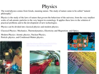
Delve into the fascinating realm of quantum mechanics with Prof. D. M. Parshuramkar as he discusses the contrast between classical and quantum mechanics. Discover how classical mechanics fails to predict the behavior of electrons in atoms and molecules, leading to the development of quantum mechanics with its unique features and equations. Explore the distinctions between particles and waves, the continuum of energy states, and the precise trajectories in classical mechanics contrasted with the uncertainty principle in quantum mechanics.

Download Presentation

Please find below an Image/Link to download the presentation.
The content on the website is provided AS IS for your information and personal use only. It may not be sold, licensed, or shared on other websites without obtaining consent from the author. Download presentation by click this link. If you encounter any issues during the download, it is possible that the publisher has removed the file from their server.
E N D
Presentation Transcript
QUANTUM MECHANICS- Illusion or Reality ? Prof. D. M. Parshuramkar Dept. of Physics N. H. College, Bramhapuri
1. Classical Mechanics Do the electrons in atoms and molecules obey Newton s classical laws of motion? We shall see that the answer to this question is No . This has led to the development of Quantum Mechanics we will contrast classical and quantum mechanics.
1.1 Features of Classical Mechanics (CM) 1) CM predicts a precise trajectory for a particle. velocityv position r = (x,y,z) The exact position (r)and velocity (v) (and hence the momentum p = mv) of a particle (mass = m) can be known simultaneously at each point in time. Note: position (r),velocity (v) and momentum (p) are vectors, having magnitude and direction v = (vx,vy,vz).
2) Any type of motion (translation, vibration, rotation) can have any value of energy associated with it i.e. there is a continuum of energy states. 3) Particles and waves are distinguishable phenomena, with different, characteristic properties and behaviour. Property Behaviour Particles Waves mass position velocity wavelength frequency momentum collisions diffraction interference
1.2 Revision of Some Relevant Equations in CM Total energy of particle: E = Kinetic Energy (KE) + Potential Energy (PE) T - depends on v V - depends on r V depends on the system e.g. positional, electrostatic PE E = mv2 + V E = p2/2m + V (p = mv) Note: strictly E, T, V (and r, v, p) are all defined at a particular time (t) E(t) etc..
Consider a 1-dimensional system (straight line translational motion of a particle under the influence of a potential acting parallel to the direction of motion): Define: position velocity momentum r = x v = dx/dt p = mv = m(dx/dt) PE force V F = (dV/dx) Newton s 2nd Law of Motion F = ma = m(dv/dt) = m(d2x/dt2) acceleration Therefore, if we know the forces acting on a particle we can solve a differential equation to determine it s trajectory {x(t),p(t)}.
1.3 Example The 1-Dimensional Harmonic Oscillator x = 0 F NB assuming no friction or other forces act on the particle (except F). k m x The particle experiences a restoring force (F) proportional to its displacement (x) from its equilibrium position (x=0). F = kx Hooke s Law k is the stiffness of the spring (or stretching force constant of the bond if considering molecular vibrations) k Substituting F into Newton s 2nd Law we get: m(d2x/dt2) = kx a (second order) differential equation
Solution: = k x(t) = Asin( t) position of particle m 1 k = /2 = frequency (of oscillation) m 2 Note: Frequency depends only on characteristics of the system (m,k) not the amplitude (A)! x time period = 1/ +A t A
Assuming that the potential energy V = 0 at x = 0, it can be shown that the total energy of the harmonic oscillator is given by: E = kA2 As the amplitude (A) can take any value, this means that the energy (E) can also take any value i.e. energy is continuous. At any time (t), the position {x(t)} and velocity {v(t)} can be determined exactly i.e. the particle trajectory can be specified precisely. We shall see that these ideas of classical mechanics fail when we go to the atomic regime (where E and m are very small) then we need to consider Quantum Mechanics. CM also fails when velocity is very large (as v c), due to relativistic effects.
1.4 Experimental Evidence for the Breakdown of Classical Mechanics By the early 20th century, there were a number of experimental results and phenomena that could not be explained by classical mechanics. a) Black Body Radiation (Planck 1900) UV Catastrophe Classical Mechanics (Rayleigh-Jeans) Energy Radiated 2000 K 1750 K 1250 K /nm 0 2000 4000 6000
Plancks Quantum Theory Planck (1900) proposed that the light energy emitted by the black body is quantized in units of h ( = frequency of light). E = nh (n = 1, 2, 3, ) High frequency light only emitted if thermal energy kT h . h a quantum of energy. h ~ 6.626 10 34 Js Planck s constant If h 0 we regain classical mechanics. Conclusions: Energy is quantized (not continuous). Energy can only change by well defined amounts.
Time period of a Simple pendulum Gustav Kirchhoff 1859 : Dark lines of Na seen in solar spectrum are darkened further by interposition of Na flame in the path of Sun s ray . Ratio of Emissive power to Absorptive power is independent of the nature of material which is
Function of Freq. and Temp. String vibration Phase Space
b) Heat Capacities (Einstein, Debye 1905-06) Heat capacity relates rise in energy of a material with its rise in temperature: CV = (dU/dT)V Classical physics Experiment At low T, heat capacity of solids determined by vibrations of solid. CV,m = 3R (for all T). CV,m < 3R (CV as T ). Einstein and Debye adopted Planck s hypothesis. Conclusion: vibrational energy in solids is quantized: vibrational frequencies of solids can only have certain values ( ) vibrational energy can only change by integer multiples of h .
c) Photoelectric Effect (Einstein 1905) h Photoelectrons ejected with kinetic energy: e Photelectrons e - Ek = h - Metal surface work function = Ideas of Planck applied to electromagnetic radiation. No electrons are ejected (regardless of light intensity) unless exceeds a threshold value characteristic of the metal. Ek independent of light intensity but linearly dependent on . Even if light intensity is low, electrons are ejected if is above the threshold. (Number of electrons ejected increases with light intensity). Conclusion: Light consists of discrete packets (quanta) of energy = photons (Lewis, 1922).
d) Atomic and Molecular Spectroscopy It was found that atoms and molecules absorb and emit light only at specific discrete frequencies spectral lines (not continuously!). e.g. Hydrogen atom emission spectrum (Balmer 1885) n1 = 1 Lyman n1 = 2 Balmer n1 = 3 Paschen n1 = 4 Brackett n1 = 5 Pfund 1 1 1 c = = = R H 2 1 2 2 n n Empirical fit to spectral lines (Rydberg-Ritz): n1, n2 (> n1) = integers. Rydberg constant RH = 109,737.3 cm-1 (but can also be expressed in energy or frequency units).
Revision: Electromagnetic Radiation wavelength A Amplitude - frequency c = x or = c / wavenumber = c= 1 / c (velocity of light in vacuum) = 2.9979 x 10⁸ m s-1.
1.5 The Bohr Model of the Atom The H-atom emission spectrum was rationalized by Bohr (1913): Energies of H atom are restricted to certain discrete values (i.e. electron is restricted to well-defined circular orbits, labelled by quantum number n). Energy (light) absorbed in discrete amounts (quanta = photons), corresponding to differences between these restricted values: E = E2 E1 = h E2 n1 p+ e n2 E2 h h E1 E1 Absorption Emission Conclusion: Spectroscopy provides direct evidence for quantization of energies (electronic, vibrational, rotational etc.) of atoms and molecules.
Limitations of Bohr Model & Rydberg-Ritz Equation The model only works for hydrogen (and other one electron ions) ignores e-e repulsion. Does not explain fine structure of spectral lines. Note: The Bohr model (assuming circular electron orbits) is fundamentally incorrect.
2. Wave-Particle Duality Remember: Classically, particles and waves are distinct: Particles characterised by position, mass, velocity. Waves characterised by wavelength, frequency. By the 1920s, however, it was becoming apparent that sometimes matter (classically particles) can behave like waves and radiation (classically waves) can behave like particles.
2.1 Waves Behaving as Particles a) The Photoelectric Effect Electromagnetic radiation of frequency can be thought of as being made up of particles (photons), each with energy E = h . This is the basis of Photoelectron Spectroscopy (PES). b) Spectroscopy Discrete spectral lines of atoms and molecules correspond to the absorption or emission of a photon of energy h , causing the atom/molecule to change between energy levels: E = h . Many different types of spectroscopy are possible.
c) The Compton Effect (1923) Experiment: A monochromatic beam of X-rays ( i) = incident on a graphite block. Observation: Some of the X-rays passing through the block are found to have longer wavelengths ( s). Intensity s i i s
Explanation: The scattered X-rays undergo elastic collisions with electrons in the graphite. Momentum (and energy) transferred from X-rays to electrons. Conclusion: Light (electromagnetic radiation) possesses momentum. p = h/ Momentum of photon E = h = hc/ Energy of photon p=h/ s s i Applying the laws of conservation of energy and momentum we get: e p=mev h ( ) ( ) = = 1 cos s i m c e
2.2 Particles Behaving as Waves Electron Diffraction (Davisson and Germer, 1925) Davisson and Germer showed that a beam of electrons could be diffracted from the surface of a nickel crystal. Diffraction is a wave property arises due to interference between scattered waves. This forms the basis of electron diffraction an analytical technique for determining the structures of molecules, solids and surfaces (e.g. LEED). NB: Other particles (e.g. neutrons, protons, He atoms) can also be diffracted by crystals.
2.3 The De Broglie Relationship (1924) In 1924 (i.e. one year before Davisson and Germer s experiment), De Broglie predicted that all matter has wave-like properties. A particle, of mass m, travelling at velocity v, has linear momentum p = mv. By analogy with photons, the associated wavelength of the particle ( ) is given by: h= h = p mv
3. Wavefunctions A particle trajectory is a classical concept. In Quantum Mechanics, a particle (e.g. an electron) does not follow a definite trajectory {r(t),p(t)}, but rather it is best described as being distributed through space like a wave. 3.1 Definitions Wavefunction ( ) a wave representing the spatial distribution of a particle . e.g. electrons in an atom are described by a wavefunction centred on the nucleus. is a function of the coordinates defining the position of the classical particle: 1-D (x) 3-D (x,y,z) = (r) = (r, , ) (e.g. atoms) may be time dependent e.g. (x,y,z,t)
The Importance of completely defines the system (e.g. electron in an atom or molecule). If is known, we can determine any observable property (e.g. energy, vibrational frequencies, ) of the system. QM provides the tools to determine computationally, to interpret and to use to determine properties of the system.
3.2 Interpretation of the Wavefunction In QM, a particle is distributed in space like a wave. We cannot define a position for the particle. Instead we define a probability of finding the particle at any point in space. The Born Interpretation (1926) The square of the wavefunction at any point in space is proportional to the probability of finding the particle at that point. Note: the wavefunction ( ) itself has no physical meaning.
1-D System If the wavefunction at point x is (x), the probability of finding the particle in the infinitesimally small region (dx) between x and x+dx is: P(x) (x) 2 dx probability density (x) the magnitude of at point x. Why write 2 instead of 2 ? Because may be imaginary or complex 2 would be negative or complex. BUT: probability must be real and positive (0 P 1). For the general case, where is complex ( = a + ib) then: 2 = * where * is the complex conjugate of . ( * = a ib) (NB ) i = 1
3-D System If the wavefunction at r = (x,y,z) is (r), the probability of finding the particle in the infinitesimal volume element d (= dxdydz) is: P(r) (r) 2 d If (r) is the wavefunction describing the spatial distribution of an electron in an atom or molecule, then: (r) 2 = (r) the electron density at point r
3.3 Normalization of the Wavefunction P(r) (r) 2 d As mentioned above, probability: What is the proportionality constant? If is such that the sum of (r) 2 at all points in space = 1, then: P(x) = (x) 2 dx P(r) = (r) 2 d 1-D 3-D As summing over an infinite number of infinitesimal steps = integration, this means: P total 2 ( ) ( ) x = = 1 D dx 1 2 2 ( ) ( ) r ( ) = = = P 3 D d x, y, z dxdydz 1 total i.e. the probability that the particle is somewhere in space = 1. In this case, is said to be a normalized wavefunction.
How to Normalize the Wavefunction 2 If is not normalized, then: ( ) r A = d 1 A corresponding normalized wavefunction ( Norm) can be defined: ( ) r Norm = 1 ( ) r A 2 ( ) r such that: = d 1 Norm The factor (1/ A) is known as the normalization constant (sometimes represented by N).
3.4 Quantization of the Wavefunction The Born interpretation of places restrictions on the form of the wavefunction: (a) must be continuous (no breaks); (b) The gradient of (d /dx) must be continuous (no kinks); (c) must have a single value at any point in space; (d) must be finite everywhere; (e) cannot be zero everywhere. Other restrictions (boundary conditions) depend on the exact system. These restrictions on mean that only certain wavefunctions and only certain energies of the system are allowed. Quantization of Quantization of E
3.5 Heisenbergs Uncertainty Principle It is impossible to specify simultaneously, with precision, both the momentum and the position of a particle* (*if it is described by Quantum Mechanics) Heisenberg (1927) px x h / 4 (or /2, where = h/2 ). x px If we know the position (x) exactly, we know nothing about momentum (px). uncertainty in position uncertainty in momentum (in the x-direction) If we know the momentum (px) exactly, we know nothing about position (x). i.e. there is no concept of a particle trajectory {x(t),px(t)} in QM (which applies to small particles). NB for macroscopic objects, x and px can be very small when compared with x and px so one can define a trajectory. Much of classical mechanics can be understood in the limit h 0.
How to Understand the Uncertainty Principle To localize a wavefunction ( ) in space (i.e. to specify the particle s position accurately, small x) many waves of different wavelengths ( ) must be superimposed large px (p = h/ ). 2 ~ 1 The Uncertainty Principle imposes a fundamental (not experimental) limitation on how precisely we can know (or determine) various observables.
Note to determine a particles position accurately requires use of short radiation (high momentum) radiation. Photons colliding with the particle causes a change of momentum (Compton effect) uncertainty in p. The observer perturbs the system. Zero-Point Energy (vibrational energy Evib 0, even at T = 0 K) is also a consequence of the Uncertainty Principle: If vibration ceases at T = 0, then position and momentum both = 0 (violating the UP). Note: There is no restriction on the precision in simultaneously knowing/measuring the position along a given direction (x) and the momentum along another, perpendicular direction (z): pz x= 0
Similar uncertainty relationships apply to other pairs of observables. e.g. the energy (E) and lifetime ( ) of a state: E. (a) This leads to lifetime broadening of spectral lines: Short-lived excited states ( well defined, small ) possess large uncertainty in the energy (large E) of the state. Broad peaks in the spectrum. (b)Shorter laser pulses (e.g. femtosecond, attosecond lasers) have broader energy (therefore wavelength) band widths. (1 fs = 10 15 s, 1 as = 10 18 s)
4. Wave Mechanics Recall the wavefunction ( ) contains all the information we need to know about any particular system. How do we determine and use it to deduce properties of the system? 4.1 Operators and Observables If is the wavefunction representing a system, we can write: Q = Q where Q observable property of system (e.g. energy, momentum, dipole moment ) operator corresponding to observable Q. Q
This is an eigenvalue equation and can be rewritten as: ( ) Q = Q function multiplied by a number Q (eigenvalue) operator Q acting on function (eigenfunction) (Note: can t be cancelled). Examples: d/dx(eax) = a eax d2/dx2 (sin ax) = a2 sin ax
To find and calculate the properties (observables) of a system: Q 1. Construct relevant operator 2. Set up equation 3. Solve equation allowed values of and Q. Q = Q Quantum Mechanical Position and Momentum Operators 1. Operator for position in the x-direction is just multiplication by x x = x d = p 2. Operator for linear momentum in the x-direction: p x = x p dx i x dx i d = p x (solve first order differential equation , px).
Constructing Kinetic and Potential Energy QM Operators 1. Write down classical expression in terms of position and momentum. 2. Introduce QM operators for position and momentum. Examples 1. Kinetic Energy Operator in 1-D T x 2 2 2 2 p p d T x x = = x= QM CM T x 2 2 m 2 m 2 m dx T 2. KE Operator in 3-D CM del-squared QM 2 2 2 2 2 2 2 2 2 p + + p p p 2 p T 2 = = + + = x y z = = T 2 2 2 2 m 2 m 2 m x y z 2 m 2 m partial derivatives operate on (x,y,z) V 3. Potential Energy Operator (a function of position) PE operator corresponds to multiplication by V(x), V(x,y,z) etc.
4.2 The Schrdinger Equation (1926) The central equation in Quantum Mechanics. Observable = total energy of system. Schr dinger Equation Hamiltonian Operator E = H H E Total Energy where T and E = T + V. H V = + SE can be set up for any physical system. The form of depends on the system. Solve SE and corresponding E. H
Examples (x) 1. Particle Moving in 1-D 2 2 2 H T V ( ) x = + = E + = V E 2 m x The form of V(x) depends on the physical situation: Free particle Harmonic oscillator V(x) = 0 for all x. V(x) = kx2 (x,y,z) 2. Particle Moving in 3-D 2 2 2 2 2 2 2 SE ( ) + + + = V x, y, z E 2 m x y z 2 ( ) or 2 + = V x, y, z E Note: The SE is a second order differential equation 2 m
4.3 Particle in a I-D Box System Particle of mass m in 1-D box of length L. Position x = 0 L. Particle cannot escape from box as PE V(x)= for x = 0, L (walls). PE inside box: V(x)= 0 for 0< x < L. 1-D Schr dinger Eqn. 2 2 PE (V) 2 = E (V = 0 inside box). 2 m x 0 L 0 x
2 2 2 = E 2 m x This is a second order differential equation with general solutions of the form: = A sin kx + B cos kx 2 2 ( ) 2 2 = + = k A sin kx B cos kx k x ( ) 2 2 2 2 2 = = SE k E 2 m 2 m x 2 2 k (i.e. E depends on k). = E 2 m
Restrictions on In principle Schr dinger Eqn. has an infinite number of solutions. So far we have general solutions: any value of {A, B, k} any value of { ,E}. BUT due to the Born interpretation of , only certain values of are physically acceptable: outside box (x<0, x>L) V = impossible for particle 2 = 0 = 0 outside box. to be outside the box must be a continuous function Boundary Conditions = 0 at x = 0 = 0 at x = L.
Effect of Boundary Conditions = A sin kx + B cos kx = B 0 1. x = 0 1 = 0 B = 0 = A sin kx for all x = A sin kL = 0 2. x = L A=0 ? (or = 0 for all x) sin kL = 0 ? kL = n sin kL = 0 n = 1, 2, 3, (n 0, or = 0 for all x)
Allowed Wavefunctions and Energies k = n /L k is restricted to a discrete set of values: n = A sin(n x/L) Allowed wavefunctions: n x = 2 sin A = (2/L) Normalization: n L L 2 2 2 2 2 k n = = E Allowed energies: n 2 2 m 2mL 2 2 n h = E n 2 8mL
Quantum Numbers There is a discrete energy state (En), corresponding to a discrete wavefunction ( n), for each integer value of n. Quantization occurs due to boundary conditions and requirement for to be physically reasonable (Born interpretation). n is a Quantum Number labels each allowed state ( n) of the system and determines its energy (En). Knowing n, we can calculate n and En.
Properties of the Wavefunction n x = 2 sin Wavefunctions are standing waves: n L L The first 5 normalized wavefunctions for the particle in the 1-D box: Successive functions possess one more half-wave ( they have a shorter wavelength). Nodes in the wavefunction points at which n = 0 (excluding the ends which are constrained to be zero). 1 0; 2 1; 3 2 Number of nodes = (n-1)


")
 Any type of motion (translation, vibration, rotation) can")


 Heat Capacities (Einstein, Debye 1905-06)")
 Photoelectric Effect (Einstein 1905)")
 Atomic and Molecular Spectroscopy")


 The Compton Effect (1923)")


")


 of a")

")