Satellite Applications in Estimating Earth's Surface Energy Budget
Satellites play a crucial role in estimating the Surface Energy Budget (SEB) by providing data on various components such as Surface Radiation Budget and Surface Turbulent Fluxes. The SEB includes factors like net radiation flux, sensible and latent heat fluxes, and subsurface heat transfer. Satellites help in assessing these fluxes and understanding land processes based on factors like surface temperature, vegetation, and radiative flux. Theoretical aspects of satellite remote sensing focus on maintaining thermal equilibrium through a combination of thermodynamic and physiological processes, balancing energy absorbed by the surface with that transferred to the atmosphere and ground.

Download Presentation

Please find below an Image/Link to download the presentation.
The content on the website is provided AS IS for your information and personal use only. It may not be sold, licensed, or shared on other websites without obtaining consent from the author. Download presentation by click this link. If you encounter any issues during the download, it is possible that the publisher has removed the file from their server.
E N D
Presentation Transcript
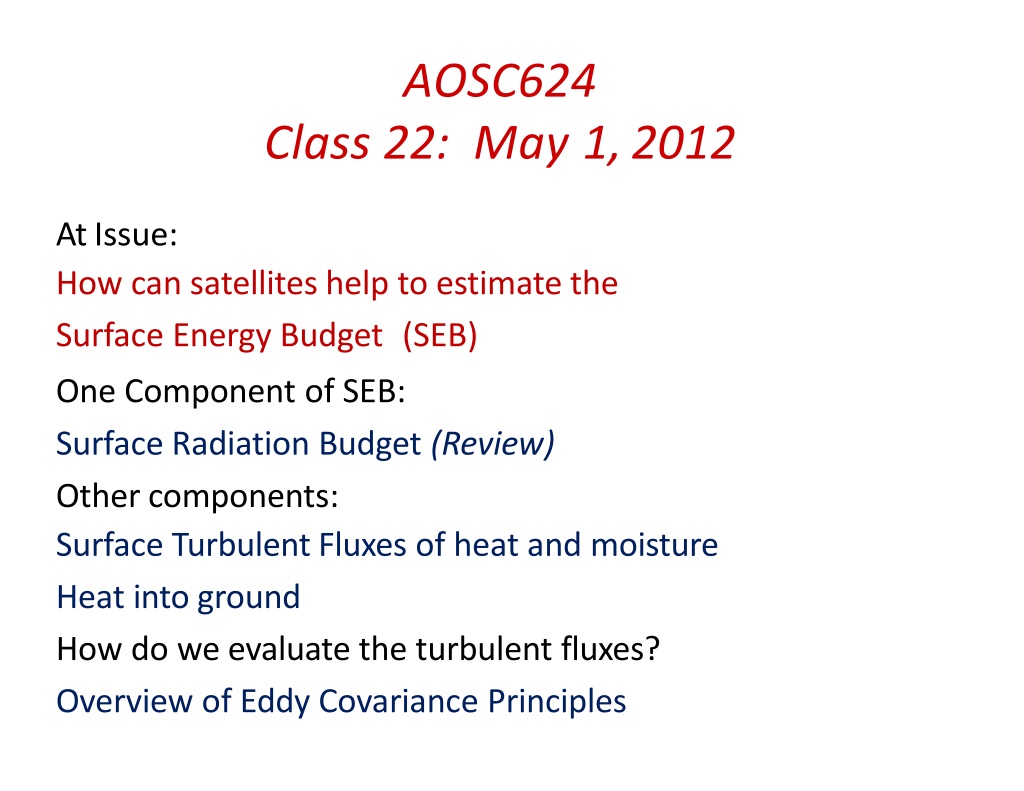
AOSC624 Class 22: May 1, 2012 AtIssue: How can satellites help to estimate the Surface Energy Budget (SEB) One Component of SEB: Surface Radiation Budget (Review) Other components: Surface Turbulent Fluxes of heat and moisture Heat into ground How do we evaluate the turbulent fluxes? Overview of Eddy Covariance Principles
Radiation Balance at the Earth Surface The net flux of radiation at the earth s surface results from a balance between the solar and terrestrial radiation fluxes: Fsfcrad = FSW +FLW The short-wave and long-wave radiation balance can beexpressed: FSW = FSW - FSW FLW = FLW -FLW The net radiation balance being: Fsfcrad = FSW - FSW + FLW - FLW
The incident solar radiation FSW is the sum of the direct and diffuse solar radiation. It has a pronounced diurnal and seasonal variation, and is also strongly affected by clouds. The outgoing short-wave solar radiation is the part reflected by the surface FSW =AsfcFSW , where Asfc is the surface albedo so that the net short-wave radiation is: FSW= (1 Asfc)FSW The outgoing long-wave radiation FLW is given by the Stefan-Boltzmann law, assuming a given emissivity for the earth s surface. The net radiation flux at the surface is then given by: Fsfcrad = FSW (1 Asfc) T4sfc+ FLW
Energy Balance at the Earth Surface The main part of the energy absorbed at the surface is used to evaporate water, another part is lost to the atmosphere as sensible heat, and a smaller part is lost to the underlying layers or used to melt snow and ice. Thus, there are essentially four types of energy fluxes at the earth s surface. They are the net radiation flux Frad, the (direct) sensible heat flux FSH , the (indirect) latent heat flux FLH , and the heat flux into the subsurface layers FG . Under steady conditions the balance equation for the energy is given by Fsfcrad - FSH - FLH - FG - FM =0
These surface fluxes are associated with land processes and depend on: vertical stability; roughness surface temperature subsurface heat conduction vegetation surface hydrological balance potential evapotranspiration radiative flux
Theoretical aspects of satellite remote sensing of energy balance Thermal equilibrium at the surface is maintained by a combination of thermodynamic and physiological processes. The net energy absorbed by the surface through radiative processes, net radiation Rn, must be balanced by that transported to the atmosphere and ground (sensible, latent, and ground heat flux): Rn = H + LE + G. (1) Rn is simply the difference between the incident and reflected shortwave radiation and the incident and emitted long wave radiation at the surface, thatis: Rn = S{1 - } + Lwd -Lwu, (2) where S is downwelling shortwave radiation energy flux (Wm-2).
Surface energy balance formulae For the sensible and latent heat components in eq. 1, closed-form solutions cannot be obtained. Commonlyused semi-empirical relationsare: For Sensible heat: H = Cp (Taero -Ta)/ra (3) sensible heat flux, W m-2; density of air, kgm-3; specific heat of air, J kg-1 oC-1; reference height air temperature,oC; Taerocanopy temperature,oC; ra aerodynamic resistance for heat and water vapor, s m-1. where H Cp Ta
In this formulation the aerodynamic resistance, ra, relates the vertical gradient in temperature, Taero - Ta, to the sensible heat flux. The ra value is semi-empirical and is intended to characterize the efficiency of the very complex transfer of heat by turbulent air movement through the canopy into the air above; ra is normally derived using empirical arguments to adjust the surface momentum transfer coefficient, a term that relates the vertical gradient in boundary layer wind speed to surface shear stress. A number of such empirical formulations are available for ra ( see Hall et al,. 1991), suchas:
ln(z 0.56h)ln[(z 0.56h) / (0.0189h)] ra =0.16U {1 + [5g(z 0.56h)(T , T ) / T U2 ]}3/4 a a aero where U is windspeed, m s-1; z is reference height for measurement of Ta and U ; h is height of canopy (m); and g is gravitational acceleration, m s-2. For more details and additional formulation for Aerodynamic Resistance see the provided paper: Measurement and estimation of the aerodynamic resistance S. Liu, D. Mao, and L. Lu
For latent heat: LE = Cp[e*(Taero)- ea)](gcga)/ (gc +ga), (5) where e*(Taero) mbar; ga s-1. These first-order solutions to the turbulent transport equations served as the primary model for investigating relationship between the properties of land surface vegetation, energy- mass balance, and remote sensing of these interactions in FIFE. ea vapor pressure at reference height, mbar; air temperature at reference height,ok; saturated vapor pressure in the canopy air space, Ta psychometric constant, mbar ok-1; as defined in (2); bulk stomatal conductance of canopy, m s-1; bulk aerodynamic conductance of canopy (1/ ra), m Cp gc
Sensibleheat For H in (3), remote sensing measures of surface radiometric temperature have been evaluated as a surrogate forTaero. However, Taerois not explicitly Tradbut, as discussed above, a theoretical construct that parameterizes a convective temperature. Vining and Blad (1991) investigated the relationship between Taeroand Trad.
Latentheat For latent heat estimation (eq. 5) the main focus of remote sensing techniques is the conductance term gc and the Taero term in estimating canopy air-space vaporpressure. The canopy conductance term gc canbe modeled after Jarvis (1976) as a product of functions with range (0, 1) where each function characterizes the dependence of gc on APAR (absorbed PAR), e, T, and leaf water potential .
Thatis: g = g (APAR)g( e)g(T c c aero)g( ) * (6) where g*(APAR) is unstressed canopy conductance and g ( e), g (Taero), g ( ) are functions with ranges (0, 1) describing the fraction of stomatal closure by vapor pressure deficit, leaf temperature, and leaf water potential. The most accurate method to estimate turbulent fluxes is the Eddy Correlation Method to be explained in what follows: c
What is Flux Flux how much of something moves through a unit area per unit time Flux is dependent on: (1) number of things crossing the area; (2) size of the area being crossed, and (3) the time it takes to cross this area
Flux Measurements Flux measurements are widely used to estimate heat, water, and CO2 exchange, as well as methane and other tracegases Eddy Covariance is one of the most direct and defensible ways to measure such fluxes The method is mathematically complex, and requires a lot of care setting up and processing data.
A Brief Practical Guide to Eddy Covariance Flux Measurements: Principles and Workflow Examples for Scientific and Industrial Applications G. Burba and D. Anderson of LI-COR Biosciences To help a non-expert gain a basic understandingof the Eddy Covariance method and to point out valuablereferences To provide explanations in a simplified manner first, and then elaborate with specificdetails
Introduction The Eddy Covariance method is one of the most accurate, direct and defensible approaches available to date for measurements of gas fluxes and monitoring of gas emissions from areas with sizes ranging from a few hundred to millions of square meters The method relies on direct and very fast measurements of actual gas transport by a 3-D wind speed in real time in situ, resulting in calculations of turbulent fluxes within the atmospheric boundary layer
Modern instruments and software makethis method easily available and potentially widely-used in studies beyond micrometeorology, such as in ecology, hydrology, environmental and industrial monitoring,etc. Main challenge of the method for a non- expert is the shear complexity of system design, implementation and processing the large volume of data
The Eddy Covariance method provides measurements of gas emission and also allows measurements of fluxes of sensible heat, latent heat and momentum, integrated over an area. This method was widely used in micrometeorology for over 30 years, but now, with firmer methodology and moreadvanced instrumentation, it can be available to any discipline, including science, industry, environmental monitoring and inventory.
Several networks have been established over the globe to measure turbulent fluxes Existing Flux Networks: Fluxnet, Fluxnet-Canada, AsiaFlux, CarboEurope and AmeriFlux networks They collect Eddy Covariance information. http://gcmd.nasa.gov/records/GCMD_AMERIFLU X_SHIDLER-CDIAC.html http://terraweb.forestry.oregonstate.edu/chair2. htm
Thereiscurrently nounifom[ or asingle methodology for EC method inology Alot of effort is being placed by networks (e.g.,Fluxnet) to unify various approaches Here we present one of the conventional ways of implementing the Eddy Covariance method
WI D Airflow canbe imaginedasahorizontalflow of numerous rotating eddies Eacheddy has3-Dcomponents,includingaverticalwindcomponent Thediagramlookschaotic but componentscanbemeasuredfromtower
time:i. eddy:i. time2 eddy2 [;J l G J G J W2 t G J air ,_ W 2 At asinglepointon the tower: Eddy 1moves parcel of air c down with thespeed w then Ed dy 2 moves parcel c2 up with the speed w2 1 1 Each pa cel has concentration,temperature, humidity; if we knowthese and the speed -we knowthe flux
Thegeneralprinciple: If we know how many molecules went up with eddies at time 1, and how many molecules went down with eddies at time 2 at the same point - we can calculate verticalflux at that point and over that time period Essenceofmethod: V ertical flux can be represented as a covariance of t he vertical velocityand concentrationofthe entityof interest
In turbulent flow, vertical flux can bepresented as: (s-p/paisthemixingratioofsubstance'cin air) F = JliliS lF=(pa +p'Q)(,..,+lt '')(s+s') Reynoldsdecomposition isused then to break into means and deviations: " Opening the parentheses: - - - F =(pa11.1s+pa - - ' pa1 pa 1v's'+p al p'a11 '+p'a1i"s + p'a11-1 ) 1 Averoged deviationfrom theavemge iszem - - - - - - Equationissimplified: F =(pali1s+pa,i,'s'+11-p'a.S' + sp'a111+ pi ',i,'s')
Nowanimportantassumptionismade(forconventionalEddy Covariance)- Le. airdensityfluctuationsareassumednegligible: ! - - - - - - Thenanother important assumptionismade- meanv rticalflow 1 s assumed negligible for horizontalhomogeneous terrain (no divergence/convergence): 'Eddy flux'
Generalequation: IF : : : : : : :Pa W ISII H = =p C ,1,'T' a Sensible heatflux: p 'l .1 \ ..1. ,../ J \f. a "'p - - , , p lt..'e /J LE = .11, Latentheatflux: Ca1 1 bondioxideflux: F l { p C ' C NOTE:Instrumentsusuallydonotmeasuremixingratios,sothereisyet p,,w's'=w''P'c anotherassumptioninthepracticalformulas(suchas:
Measurementsatapointcanrepresentanupwindarea Measurementsaredoneinsidethe boundary layerof interest Fetch/footprint is adequate-fluxes are measured only at the area of interest Flux isfullyturbulent -most of the netverticaltransfer is done byeddies Terrainis horizontaland unitorm: averageof fluctuations iszero; airdensityfluctuations,flow convergence & divergence arenegligible Instrumentscandetect verysmall changes at very highfrequency r - I
Measurements are not perfect:due to assumptions,physical phenomena,instrument problems,andspecificitiesofterrainandsetup There could be a number of flux errors introduced if not corrected: Other key errorsources: Systemtime response Sensorseparation Sc arpa haver- ,ing ube 11KllDR .,.,..._ c r lon
Theseerrorsarenottrivial-they maycombinetoover10o%ofthe flux Tominimizeoravoidsucherrorsanumberofprocedurescouldbeperformed Affected fluxes Approximate Range Errorsdue to Frequencyresponse all 5-30% all T mederay 5-15% all Spikes,nose 0-15% Unleveledmstrument/flow all 0-25% H20,co>'CH.. sensibleheat Densityfluctuatton 0-50% Sonic heaterror 0..10% BandBroadeningfor NDtR mostlyC03 0..5% 0 3o96 Spectroscop..:effect forLASER anygas someH30 0 1096 Oxygen ln thepath all O Messing data fillIng
Errors Remedy frequency respo secorrections Fruency respose Time lay adjust g for delay Spikes,noise spikeremoval coord ate rotatio Unleveled inst1ument/ ow Densityfluctuation Webb..Pearman Leun ng correction Son c heaterror sonctemperature correction Ba d Broaden g forNDIR nd..broadeningcorrectton SpKtroscopic effect forLASER no uniform W1dely usedcorrecnon Oxyge int e path oxygencorrect on Miss g datafill ng Methodology/tests: Monte-Carloetc-
Measuresfluxestransported byeddies Requiresturbulent flow Requiresstate-of-the-artinstruments Calculated ascovariance of w' and c' Many assumptions to satisfy Complex calculations Most direct wayto measureflux Continuousnewdevelopments
TERRESTRIAL OCEANOGRAPHIC <1%of apphcabOns 98%of applications <1%ofapplications May needcustomized Designed forstafonary use May needcustomized reinforcement coating,LPS3 Limited byprecipitation, fog,&dew May be affected by extreme temperaturesand vibrations May be affected by precipitation,dew,& gyroscopiceffects
The power consumption bythe entire EddyCovariance station inthe Florida Everglades ,Ll-7500for C0:1/H20,some anemometer,and was<30Watts,includingLl-nooforCH4 airtemperature/relative humidity sensorsand barometer The 1 2 lb.(5.5kg)open pathmethaneanatyzerwas carried Intothewetland by onepersoninthe backpack,alongwithtools,othersensors,andalaptop Insuch remoteplacesoccasionalcalibrationcheckscanbedoneusingsmall hand-earned gastankswithknownCH4concentration andCH4-freeair
Remote sensing the surface energy budget The First International Satellite Land Surface Climatology Project (ISLSCP) Field Experiment (FIFE) was an international, land-surface-atmosphere experiment centered on a 15 x 15 km test site near Manhattan,Kansas. The objectives ofFIFE: to better understand the role of biology in controlling the interactions between the atmosphere and the vegetated land surface and to investigate the use of satellite observations for inferring climatologically significant land surface parameters. Specifically:
to verify the basic flux relationships for the homogeneous patches; to assess the ability to remotely sense parametric inputs to theserelationships; to examine how these relationships and remote sensing algorithms scale from the patch level to heterogeneous collections of patches at the meso- scalelevel; to determine how well existing calibration, atmospheric correction, and radiometric rectification techniques permit to extend satellite observations between dates andsensors to determine to what degree existing and future satellite designs satisfy the requirements for periodic monitoring of surface energy balance components on a globalscale.
Below are a few examples of the sources of information on the various methods of flux measurements, and specifically on the Eddy Covariance method: Micrometeorology, 2009. By T. Foken. Springer-Verlag. Handbook of Micrometeorology: A Guide for Surface Flux Measurement and Analysis, 2008. By X. Lee; W. Massman; B. Law (Eds.). Springer-Verlag. Principles of Environmental Physics, 2007. By J. Monteith and M. Unsworth. AcademicPress. Microclimate: The Biological Environment. 1983. By N. Rosenberg, B. Blad, S. Verma. WileyPublishers. Baldocchi, D.D., B.B. Hicks and T.P. Meyers. 1988. 'Measuring biosphere- atmosphere exchanges of biologically related gases with micrometeorological methods', Ecology, 69, 1331-1340 Verma, S.B., 1990. Micrometeorological methods for measuring surface fluxes of mass and energy. Remote Sensing Reviews, 5: 99-115. Wesely, M.L., D.H. Lenschow and O.T. 1989. Flux measurement techniques. In: Global Tropospheric Chemistry, Chemical Fluxes in the Global Atmosphere. NCAR Report. Eds. DH Lenschow and BB Hicks. pp 31-46


ln[(z − 0.56h) / (0.0189h)]")