Understanding the Binomial Option Pricing Model


Chapter - 4
Option Pricing Models
The Binomial Model
1

•
This chapter examines the first of two type of option
pricing model. A
model
is a simplified representation
of reality that uses certain inputs to produce an
output, or result.
•
An
option pricing model
is a mathematical formula
or computational procedure that uses the factors
determining the option's price as inputs. The output is
the theoretical fair value of the option.
2
•
If the model performs as it should, the option's market
price will equal the theoretical fair value.
•
Obtaining the theoretical fair value is a process called
option pricing
.
3
•
We begin with a simple model called the
binomial
pricing model
, we move on to Chapter 5 and the
Black-Scholes-Merton option pricing model
.
•
In both cases, we have the same objective: to obtain
the theoretical fair value of the option, which is the
price at which it should be trading.
4
One-Period Binomial Model
•
We will assume that the option’s European life is a single time
period. Consider a world in which there is a stock priced at S
on which call option are available .
•
The call has one period remaining before it expires. The
beginning of the period is today and is referred to as time 0.
The end of the period is referred to as time 1.
•
When the call expires, the stock can take on one of two values.
It can go up by a factor of u or down by a factor of d.
5
•
If it goes up, the stock price will be uS. If it goes
down, it will be Ds.
•
For example, suppose that the stock price is currently
$50 and can go either up by 10 percent or down by8
percent. Thus, u=(10/100)+1=1.1 and d= (8/100)-
1=0.92. when the call expires, the stock will be either
50(1.1)=55 or 50(0.92)=46.
6
•
Consider a call option on the stock with an exercise
price of X and a current price of C. When the option
expires, it will be worth either C
u
or C
d
. Because at
expiration the call price is its intrinsic value, then
Cᵤ = Max. [0, uS – X]
C
d
= Max. [0, dS – X]
•
Next two figures illustrates the paths of both the stock
and the call prices.
7
The One Period Binomial Tree
A - The Stock Price Path
Time 0
Time 1
uS
S
dS
8
The One Period Binomial Tree
B - The Call Price Path
Time 0
Time 1
C
ᵤ
C
C
d
9
•
Let the per period risk-free rate be identified by the
symbol r. the risk-free rate is the interest earned on a
riskless investment over a time period equal to the
option’s remaining life.
•
The risk-free rate is between the rate of return if the
stock goes up and the rate of return if the stock goes
down. Thus, d < 1 + r < u.
10
•
The objective of this model is to drive a formula for
the theoretical fair value of the option, the variable C.
•
The formula for C is developed by constructing a
riskless portfolio of stock and options.
•
This riskless portfolio is called a hedge portfolio and
consists of h shares of stock and written calls.
11
•
The current value of the portfolio is the value of the h
shares minus the value of the short call.
Why we subtract the call’s value from the value of the
shares?????
•
Denoted as V, where V = hS – C, is the amount of our
own money required to construct the hedge portfolio.
•
V
u
= huS – C
u
, V
d
= hdS – C
d
•
The model provides the hedge ratio, h .
h =
C
ᵤ -
C
d
uS- dS
12
C = pC
ᵤ + (1 – p )
C
d
1 + r
Where: p is defined as (1 + r – d) / (u – d)
r risk-free rate
13
•
Which variables affecting the call option parameters??
•
The one-period binomial option pricing formula
provides the option price as a weighted average of the
two possible option prices at expiration, discounted at
the risk-free rate.
14
Example 1:
Consider a stock currently priced at $100. One
period later it can go up to $125, an increase of 25
percent, or down to $80, a decrease of 20 percent.
Assume a call option with an exercise price of $100. The
risk-free rate is 7 percent .Calculate the C and h.
The inputs are summarized as follows:
S = 100 d = 0.80
X =100 r = 0.07
u = 1.25
15
•
First, we find the values of Cᵤ and Cd
:
C
ᵤ = Max[0, uS –X]
= Max[0,100(1.25)-100]
= 25
C
d
= Max[0, dS –X]
= Max[0,100(0.80)-100]
= 0
h = ( 25 – 0 ) / ( 125 – 80 )
= 0.556
16
P =
(1 + r – d) / (u – d)
= 1.07 – 0.80 = 0.6
1.25 – 0.80
C = pC
ᵤ + (1 – p )
C
d
1 + r
= (0.6) 25 + (0.4)0
1.07
= 14.02
Thus, the theoretical fair value of the call is 14.02.
17
•
Consider a hedge portfolio consisting of 1,000 calls and
556 shares of stock. The number of shares is determined
by the hedge ratio of 0.556 shares per written call.
•
The current value of the hedge portfolio is
556($100) – 1,000($14.02)
$55,600 – $14,020 =
$41,580
•
This total represents the assets (the stock) minus the
liabilities (the calls), and thus is the net worth, or the
amount the investor must commit to the transaction.
18
•
If the stock goes up to $125,
the call will exercised for a value of
$125-$100 = $25.
The stock will be worth 556($125) = $69,500.
The hedge portfolio will be worth
556($125) – 1000($125 - $100) = $44,500.
•
If the stock goes down to $80,
the call will be expire out-of-the-money.
The hedge portfolio will be worth
556($80)= $44,480.
19
•
These two values of the hedge portfolio at expiration
are essentially equal, because the $20 difference is
due only to the rounding off of the hedge ratio. The
return on the hedge portfolio is :
r
h
= $44,500 - 1
≈
0.07
$41,580
which is the risk-free rate.
•
The original investment of $41,580 will have grown
to $44,500 a return of about 7 percent, the risk-free
rate.
20
One-Period Binomial Example
uS=$125
C
u
=25
V
u
=556(125)-1,000(25) =44,500
r
h
=(44,500/41,580)-1≈0.07
S = $100
h = 0.556
Hold 556 shares @$100,
1,000 calls@$14.02
V=556(100)-1,000(14.02)= 41,580
dS=$80
C
d
=0
V
d
=556(80)-1000(0)=44,480
r
h
=(44,480/41,580)-1≈0.07
21
Two Period Binomial Model
•
In the single-period world, the stock price goes either
up or down. Thus, there are only two possible future
stock price. To increase the degree of realism, we will
now add another period. This will increase the
number of possible outcomes at expiration.
22
Time 0 Time 1 Time2
u²S
uS
S
udS
dS
d²S
23
The Two-Period Binomial Tree
a-The Stock Price Path
b-The Call Price Path
Time 0 Time 1 Time2
C
ᵤ
²
C
ᵤ
C
C
ᵤ
d
C
d
C
d
²
24
•
The option prices at expiration are:
C
ᵤ
²
= Max[0, u²S – X]
C
ᵤ
d
=
Max[0, udS – X]
C
d
²
= Max[0, d²S – X]
C
ᵤ = p
C
ᵤ
²
+ (1- p)
C
ᵤ
d
C
d
= p
C
ᵤ
d
+ (1- p)
C
d
²
1+ r 1 + r
C = p
² C
ᵤ
²
+ 2p(1 – p)C
ᵤ
d
+ (1 – p)
² C
d
²
( 1 + r)
²
25
•
The two-period binomial option pricing formula
provides the option price as a weighed average of the
two possible option prices the next period, discounted
at the risk-free rate. The two future option prices are
obtained from the one-period binomial model.
26
Example 2:
Consider the previous example with two-period all
inputs values remain the same.
Calculate the value of the call option and the hedge
ratio.
27
•
The possible stock prices at expiration are:
u²S = 100(1.25)
² = 156.25
udS = 100(1.25)(0.8) = 100
d²S = 100(0.8)
² = 64
•
The call prices at expiration are:
C
ᵤ
² = Max[0, u²S – X]
= Max(0,156.25-100) = 56.25
C
ᵤ
d
=
Max[0, udS – X]
= Max(0,100-100) = 0
C
d
²
= Max[0, d²S – X]
= Max(0,64-100) = 0
28
•
C
ᵤ = p
C
ᵤ
² + (1- p) C
ᵤd
1+r
= (0.6)56.25+(0.4)0 = 31.54
1.07
•
C
d
= p
C
ᵤ
d
+ (1- p)
C
d
²
1+r
= (0.6)0+(0.4)0 = 0
1.07
•
C =
p
² C
ᵤ
²
+ 2p(1 – p)C
ᵤ
d
+ (1 – p)
² C
d
²
( 1 + r)
²
= (0.6)31.54+(0.4)0 = 17.69
1.7
29
؞
The value of the call at time 0 is a weighted average of
the two possible call values one period later.
•
Note that the same call analyzed in the one-period
world is worth more in the two period world. Why??
Recall from Chapter 3 that a call option with a
longer maturity is never worth less than one with a
shorter maturity and usually is worth more.
30
Pricing Put Option
•
We can use the binomial model to price put options
just as we can for call options. We can use the same
formulas, but instead of specifying the call payoffs at
expiration, we use the put payoffs at expiration. Then
simply replace every C with a P in each formula.
31
•
P = p
² P
ᵤ
² + 2p(1 – p)P
ᵤ
d
+ (1 – p)
² P
d
²
( 1 + r)
²
•
P = pP
ᵤ + (1 – p )
P
d
1 + r
•
P
ᵤ = p
P
ᵤ
²
+ (1- p) P
ᵤ
d
P
d
= p
P
ᵤ
d
+ (1- p)
P
d
²
1+ r 1 + r
32
•
Pricing a put with the binomial model is the same
procedure as pricing a call, except that the expiration
payoffs reflect the fact that the option is the right to
sell the underlying stock.
33
American Puts and Early Exercise
•
Let us use the same two-period put with an exercise
price of 100 but make it an American put. This means
that at any point in the life of the option, we can
choose to exercise it early if it is best to do, So that
means at any point in the binomial tree when the put
is in-the-money.
34
•
For example, go back to the values calculated for the
European put at time 1. recall that they were
P
u
= (0.6)0 – (0.4)0 = 0, when the stock is at 125
1.07
P
d
= (0.6)0 – (0.4)36 = 13.46, when the stock is at 80
1.07
•
When the stock is at 125 the put is out-of-the-money,
so we do not need to worry about exercising it. When
the stock is at 80 the put is in-the-money by $20,
which is far more than its unexercised value of $13.46.
35
•
So we exercise it, which means that we replace the
calculated value P
d
of13.46 with 20. Thus, we now
have P
u
=0 and P
d
=20. Then the value at time 0 is
P = (0.6)0 – (0.4)20 = 7.48
1.07
•
The binomial model can easily accommodate the
early exercise of an American put by simply replacing
the computed value with the intrinsic value if the
latter is greater.
36
Binomial Option Pricing Model Advantages
•
It is useful for valuing derivatives such as American
options which allow the owner to exercise the option
at any point in time until expiration (unlike European
options which are exercisable only at expiration).
•
The model is also somewhat simple mathematically
when compared to counterparts such as the Black-
Scholes model, and is therefore relatively easy to
build and implement with a computer spreadsheet.
37
•
Perhaps the most valuable feature of the model is that
it enables you to see how the construction of a
dynamic risk-free hedge leads to a formula for the
option price.
38
This chapter delves into the fundamental concept of option pricing models, specifically focusing on the Binomial Model. An option pricing model serves as a mathematical framework to calculate the fair value of an option based on certain inputs. The ultimate goal is to determine the theoretical fair value of an option through a process known as option pricing. The one-period Binomial Model is explored in detail, illustrating how it can be used to evaluate European call options in a simple yet effective manner.

Download Presentation

Please find below an Image/Link to download the presentation.
The content on the website is provided AS IS for your information and personal use only. It may not be sold, licensed, or shared on other websites without obtaining consent from the author. Download presentation by click this link. If you encounter any issues during the download, it is possible that the publisher has removed the file from their server.
E N D
Presentation Transcript
Chapter - 4 Option Pricing Models The Binomial Model 1
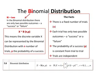
This chapter examines the first of two type of option pricing model. A model is a simplified representation of reality that uses certain inputs to produce an output, or result. An option pricing model is a mathematical formula or computational procedure that uses the factors determining the option's price as inputs. The output is the theoretical fair value of the option. 2
If the model performs as it should, the option's market price will equal the theoretical fair value. Obtaining the theoretical fair value is a process called option pricing. 3
We begin with a simple model called the binomial pricing model , we move on to Chapter 5 and the Black-Scholes-Merton option pricing model. In both cases, we have the same objective: to obtain the theoretical fair value of the option, which is the price at which it should be trading. 4
One-Period Binomial Model We will assume that the option s European life is a single time period. Consider a world in which there is a stock priced at S on which call option are available . The call has one period remaining before it expires. The beginning of the period is today and is referred to as time 0. The end of the period is referred to as time 1. When the call expires, the stock can take on one of two values. It can go up by a factor of u or down by a factor of d. 5
If it goes up, the stock price will be uS. If it goes down, it will be Ds. For example, suppose that the stock price is currently $50 and can go either up by 10 percent or down by8 percent. Thus, u=(10/100)+1=1.1 and d= (8/100)- 1=0.92. when the call expires, the stock will be either 50(1.1)=55 or 50(0.92)=46. 6
Consider a call option on the stock with an exercise price of X and a current price of C. When the option expires, it will be worth either Cu or Cd. Because at expiration the call price is its intrinsic value, then C = Max. [0, uS X] Cd = Max. [0, dS X] Next two figures illustrates the paths of both the stock and the call prices. 7
The One Period Binomial Tree A - The Stock Price Path Time 0 Time 1 uS S dS 8
The One Period Binomial Tree B - The Call Price Path Time 0 Time 1 C C Cd 9
Let the per period risk-free rate be identified by the symbol r. the risk-free rate is the interest earned on a riskless investment over a time period equal to the option s remaining life. The risk-free rate is between the rate of return if the stock goes up and the rate of return if the stock goes down. Thus, d < 1 + r < u. 10
The objective of this model is to drive a formula for the theoretical fair value of the option, the variable C. The formula for C is developed by constructing a riskless portfolio of stock and options. This riskless portfolio is called a hedge portfolio and consists of h shares of stock and written calls. 11
The current value of the portfolio is the value of the h shares minus the value of the short call. Why we subtract the call s value from the value of the shares????? Denoted as V, where V = hS C, is the amount of our own money required to construct the hedge portfolio. Vu = huS Cu, Vd= hdS Cd The model provides the hedge ratio, h . h = C - Cd uS- dS 12
C = pC + (1 p ) Cd 1 + r Where: p is defined as (1 + r d) / (u d) r risk-free rate 13
Which variables affecting the call option parameters?? The one-period binomial option pricing formula provides the option price as a weighted average of the two possible option prices at expiration, discounted at the risk-free rate. 14
Example 1: Consider a stock currently priced at $100. One period later it can go up to $125, an increase of 25 percent, or down to $80, a decrease of 20 percent. Assume a call option with an exercise price of $100. The risk-free rate is 7 percent .Calculate the C and h. The inputs are summarized as follows: S = 100 d = 0.80 X =100 r = 0.07 u = 1.25 15
First, we find the values of C and Cd : C = Max[0, uS X] = Max[0,100(1.25)-100] = 25 Cd = Max[0, dS X] = Max[0,100(0.80)-100] = 0 h = ( 25 0 ) / ( 125 80 ) = 0.556 16
P = (1 + r d) / (u d) = 1.07 0.80 = 0.6 1.25 0.80 C = pC + (1 p ) Cd 1 + r = (0.6) 25 + (0.4)0 1.07 = 14.02 Thus, the theoretical fair value of the call is 14.02. 17
Consider a hedge portfolio consisting of 1,000 calls and 556 shares of stock. The number of shares is determined by the hedge ratio of 0.556 shares per written call. The current value of the hedge portfolio is 556($100) 1,000($14.02) $55,600 $14,020 = $41,580 This total represents the assets (the stock) minus the liabilities (the calls), and thus is the net worth, or the amount the investor must commit to the transaction. 18
If the stock goes up to $125, the call will exercised for a value of $125-$100 = $25. The stock will be worth 556($125) = $69,500. The hedge portfolio will be worth 556($125) 1000($125 - $100) = $44,500. If the stock goes down to $80, the call will be expire out-of-the-money. The hedge portfolio will be worth 556($80)= $44,480. 19
These two values of the hedge portfolio at expiration are essentially equal, because the $20 difference is due only to the rounding off of the hedge ratio. The return on the hedge portfolio is : rh = $44,500 - 1 0.07 $41,580 which is the risk-free rate. The original investment of $41,580 will have grown to $44,500 a return of about 7 percent, the risk-free rate. 20
One-Period Binomial Example uS=$125 Cu=25 Vu=556(125)-1,000(25) =44,500 rh=(44,500/41,580)-1 0.07 S = $100 h = 0.556 Hold 556 shares @$100, 1,000 calls@$14.02 V=556(100)-1,000(14.02)= 41,580 dS=$80 Cd=0 Vd=556(80)-1000(0)=44,480 rh=(44,480/41,580)-1 0.07 21
Two Period Binomial Model In the single-period world, the stock price goes either up or down. Thus, there are only two possible future stock price. To increase the degree of realism, we will now add another period. This will increase the number of possible outcomes at expiration. 22
The Two-Period Binomial Tree a-The Stock Price Path Time 0 Time 1 Time2 u S uS S udS dS d S 23
b-The Call Price Path Time 0 Time 1 Time2 C C CC d Cd Cd 24
The option prices at expiration are: C = Max[0, u S X] C d = Max[0, udS X] Cd = Max[0, d S X] C = p C + (1- p) C dCd = pC d + (1- p) Cd 1+ r 1 + r C = p C + 2p(1 p)C d+ (1 p) Cd ( 1 + r) 25
The two-period binomial option pricing formula provides the option price as a weighed average of the two possible option prices the next period, discounted at the risk-free rate. The two future option prices are obtained from the one-period binomial model. 26
Example 2: Consider the previous example with two-period all inputs values remain the same. Calculate the value of the call option and the hedge ratio. 27
The possible stock prices at expiration are: u S = 100(1.25) = 156.25 udS = 100(1.25)(0.8) = 100 d S = 100(0.8) = 64 The call prices at expiration are: C = Max[0, u S X] = Max(0,156.25-100) = 56.25 C d = Max[0, udS X] = Max(0,100-100) = 0 Cd = Max[0, d S X] = Max(0,64-100) = 0 28
C = p C + (1- p) Cd 1+r = (0.6)56.25+(0.4)0 = 31.54 1.07 Cd = pC d + (1- p) Cd 1+r = (0.6)0+(0.4)0 = 0 1.07 C = p C + 2p(1 p)C d + (1 p) Cd ( 1 + r) = (0.6)31.54+(0.4)0 = 17.69 1.7 29
The value of the call at time 0 is a weighted average of the two possible call values one period later. Note that the same call analyzed in the one-period world is worth more in the two period world. Why?? Recall from Chapter 3 that a call option with a longer maturity is never worth less than one with a shorter maturity and usually is worth more. 30
Pricing Put Option We can use the binomial model to price put options just as we can for call options. We can use the same formulas, but instead of specifying the call payoffs at expiration, we use the put payoffs at expiration. Then simply replace every C with a P in each formula. 31
P = p P + 2p(1 p)Pd + (1 p) Pd ( 1 + r) P = pP + (1 p ) Pd 1 + r P = p P + (1- p) P dPd = pP d + (1- p) Pd 1+ r 1 + r 32
Pricing a put with the binomial model is the same procedure as pricing a call, except that the expiration payoffs reflect the fact that the option is the right to sell the underlying stock. 33
American Puts and Early Exercise Let us use the same two-period put with an exercise price of 100 but make it an American put. This means that at any point in the life of the option, we can choose to exercise it early if it is best to do, So that means at any point in the binomial tree when the put is in-the-money. 34
For example, go back to the values calculated for the European put at time 1. recall that they were Pu = (0.6)0 (0.4)0 = 0, when the stock is at 125 1.07 Pd = (0.6)0 (0.4)36 = 13.46, when the stock is at 80 1.07 When the stock is at 125 the put is out-of-the-money, so we do not need to worry about exercising it. When the stock is at 80 the put is in-the-money by $20, which is far more than its unexercised value of $13.46. 35
So we exercise it, which means that we replace the calculated value Pd of13.46 with 20. Thus, we now have Pu=0 and Pd=20. Then the value at time 0 is P = (0.6)0 (0.4)20 = 7.48 1.07 The binomial model can easily accommodate the early exercise of an American put by simply replacing the computed value with the intrinsic value if the latter is greater. 36
Binomial Option Pricing Model Advantages It is useful for valuing derivatives such as American options which allow the owner to exercise the option at any point in time until expiration (unlike European options which are exercisable only at expiration). The model is also somewhat simple mathematically when compared to counterparts such as the Black- Scholes model, and is therefore relatively easy to build and implement with a computer spreadsheet. 37
Perhaps the most valuable feature of the model is that it enables you to see how the construction of a dynamic risk-free hedge leads to a formula for the option price. 38


 Cd")


 / (u – d)")


 Cᵤd")


Pᵤd + (1 – p)² Pd²")