Understanding B+ Tree Basics and Design in Data Structures

Explore the fundamentals of B+ trees in this lecture, covering topics like tree parameter definitions, internal and leaf nodes, page formatting, search processes, and insertion techniques. Discover how B+ trees organize and retrieve data efficiently, making them an essential data structure in database systems and file management.

Uploaded on Oct 03, 2024 | 0 Views
Download Presentation

Please find below an Image/Link to download the presentation.
The content on the website is provided AS IS for your information and personal use only. It may not be sold, licensed, or shared on other websites without obtaining consent from the author. Download presentation by click this link. If you encounter any issues during the download, it is possible that the publisher has removed the file from their server.
E N D
Presentation Transcript
Lecture 13 Lecture 13 Lecture 13: B+ Tree (continued)
Lecture 13 Lecture 13 What you will learn about in this section 1. Recap: B+ Trees 2. B+ Trees: Cost 3. B+ Trees: Clustered 2
Lecture 13 Lecture 13 1. Recap: B+ Trees 3
Lecture 13 > Section 2 > B+ Tree basics Lecture 13 > Section 2 > B+ Tree basics B+ Tree Basics Parameter d d = the order Each non-leaf ( interior ) node has d ? 2d entries Minimum 50% occupancy Minimum 50% occupancy node 10 20 30 entries node has 1 ? 2d Root node entries entries
Lecture 13 > Section 2 > B+ Tree basics Lecture 13 > Section 2 > B+ Tree basics B+ Tree Basics Non-leaf or internal node 10 20 30 Leafnodes 32 34 37 38 12 17 22 25 28 29 Name: Sally Age: 28 Name: Sue Age: 33 Name: Jake Age: 15 Name: Bess Age: 22 Name: Jess Age: 35 Name: Alf Age: 37 Name: Joe Age: 11 Name: John Age: 21 Name: Bob Age: 27 Name: Sal Age: 30
Lecture 13 > Section 2 > B+ Tree basics Lecture 13 > Section 2 > B+ Tree basics B+ Tree Page Format index entries Non-leaf P1 K1 Pm P2 K2 KmPm+1 P3 Page Pointer to a page with values Km Pointer to a page with Values < K1 Pointer to a page with values s.t. K1 Values < K2 Pointer to a page with values s.t., K2 Values < K3 data entries Leaf Page R1 K1 P0 R2 K2 Pn+1 Rn Kn Next Page Pointer Prev Page Pointer record 1 record 2 record n
Lecture 13 > Section 3 > B+ Tree design & cost B+ Tree: Search start from root examine index entries in non-leaf nodes to find the correct child traverse down the tree until a leaf node is reached non-leaf nodes can be searched using a binary or a linear search
Lecture 13 > Section 3 > B+ Tree design & cost B+ Tree: Insert Find correct leaf L. Put data entry onto L. If L has enough space, done! Else, must splitL (into L and a new node L2) Redistribute entries evenly, copy up middle key. Insert index entry pointing to L2 into parent of L. This can happen recursively To split non-leaf node, redistribute entries evenly, but pushing up the middle key. (Contrast with leaf splits.) Splits grow tree; root split increases height. Tree growth: gets wider or one level taller at top.
Lecture 13 > Section 3 > B+ Tree design & cost B+ Tree: Deleting a data entry Start at root, find leaf L where entry belongs. Remove the entry. If L is at least half-full, done! If L has only d-1 entries, Try to re-distribute, borrowing from sibling (adjacent node with same parent as L). If re-distribution fails, mergeL and sibling. If merge occurred, must delete entry (pointing to L or sibling) from parent of L. Merge could propagate to root, decreasing height.
Lecture 13 Lecture 13 2. B+ Trees: Cost 10
Lecture 13 > Section 2 > B+ Tree cost Lecture 13 > Section 2 > B+ Tree cost B+ Tree: High Fanout = Smaller & Lower IO As compared to e.g. binary search trees, B+ Trees have highfanout (between d+1 and 2d+1) The fanout fanout is defined as the number of pointers to child nodes coming out of a node This means that the depth of the tree is small getting to any element requires very few IO operations! Also can often store most or all of the B+ Tree in main memory! Note that Note that fanout we ll often assume it s constant we ll often assume it s constant just to come up with approximate just to come up with approximate eqns eqns! ! fanout is dynamic is dynamic- - A TiB = 240 Bytes. What is the height of a B+ Tree (with fill-factor = 1) that indexes it (with 64K pages)? (2*2730 + 1)h = 240 h = 4
Lecture 13 > Section 2 > B+ cost Lecture 13 > Section 2 > B+ cost Simple Cost Model for Search Let: f = fanout, which is in [d+1, 2d+1] (we ll assume it s constant for our cost model ) N = the total number of pages we need to index F = fill-factor (usually ~= 2/3) Our B+ Tree needs to have room to index N / F pages! We have the fill factor in order to leave some open slots for faster insertions What height (h) does our B+ Tree need to be? h=1 Just the root node- room to index f pages h=2 f leaf nodes- room to index f2 pages h=3 f2 leaf nodes- room to index f3 pages h fh-1 leaf nodes- room to index fh pages! We need a B+ Tree of height h = log? ? ?!
Lecture 13 > Section 2 > B+ cost Lecture 13 > Section 2 > B+ cost Simple Cost Model for Search Note that if we have B available buffer pages, by the same logic: We can store ?? levels of the B+ Tree in memory where ??is the number of levels such that the sum of all the levels nodes fit in the buffer: ? 1 + ? + + ??? 1= ?=0 ?? 1?? ? ? ??+ 1 In summary: to do exact search: We read in one page per level of the tree However, levels that we can fit in buffer are free! Finally we read in the actual record IO Cost: log? ?? 1?? where ? ?=0
Lecture 13 > Section 2 > B+ Tree cost Lecture 13 > Section 2 > B+ Tree cost Simple Cost Model for Search To do range search, we just follow the horizontal pointers The IO cost is that of loading additional leaf nodes we need to access + the IO cost of loading each page of the results- we phrase this as Cost(OUT) ? ? ??+ ????(???) IO Cost: log? ?? 1?? where ? ?=0
Lecture 13 Lecture 13 3. B+ Trees: Clustered 15
Lecture 13 > Section 3 Clustered Indexes An index is clustered if the underlying data is ordered in the same way as the index s data entries.
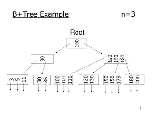
Lecture 13 > Section 3 Clustered vs. Unclustered Index 30 30 Index Entries 32 34 37 38 32 34 37 38 22 25 28 29 22 25 28 29 37 19 22 37 19 33 22 28 30 33 35 35 30 27 27 28 Data Records Clustered Unclustered
Lecture 13 > Section 3 Clustered vs. Unclustered Index Recall that for a disk with block access, sequential IO is much faster than random IO For exact search, no difference between clustered / unclustered For range search over R values: difference between 1 random IO + R sequential IO, and R random IO: A random IO costs ~ 10ms (sequential much much faster) For R = 100,000 records- difference between ~10ms and ~17min!
Lecture 13 > SUMMARY Lecture 13 > SUMMARY Summary We create indexes over tables in order to support fast (exact and range) search and insertion over multiple search keys B+ Trees are one index data structure which support very fast exact and range search & insertion via high fanout Clustered vs. unclustered makes a big difference for range queries too
Lecture 14 Lecture 14 Lecture 14: Hash Indexes
Lecture 14 Lecture 14 What you will learn about in this section 1. Hash Indexes 2. Static Hashing 3. Extendible Hashing 21
Lecture 14 Lecture 14 1. Hash Indexes 22
Lecture 14 > Section 1 Hash Index A hash index is a collection of buckets bucket = primary page plus overflow pages buckets contain one or more data entries uses a hash function h h(r) = bucket in which (data entry for) record r belongs
Lecture 14 > Section 1 Hash Index A hash index is: good for equality search not so good for range search (use tree indexes instead) Types of hash indexes: Static hashing Extendible hashing (dynamic) Linear hashing (dynamic) not covered in the course, see 11.3 in the cow book
Lecture 14 > Section 1 Operations on Hash Indexes Equality search apply the hash function on the search key to locate the appropriate bucket search through the primary page (plus overflow pages) to find the record(s) Deletion find the appropriate bucket, delete the record Insertion find the appropriate bucket, insert the record if there is no space, create a new overflow page
Lecture 14 > Section 1 Hash Functions An ideal hash function must be uniform: each bucket is assigned the same number of key values A bad hash function maps all search key values to the same bucket Examples of good hash functions: h(k) = a * k + b, where a and b are constants a random function
Lecture 14 Lecture 14 2. Static Hashing 27
Lecture 14 > Section 2 Static Hashing # primary bucket pages fixed, allocated sequentially, never de-allocated; overflow pages if needed. h(k) mod N = bucket to which data entry withkey k belongs. (N = # of buckets) 0 h(key) mod N key 1 h N-1 Primary bucket pages Overflow pages
Lecture 14 > Section 2 Static Hashing: Example 4 buckets each bucket has 2 data entries (full record) overflow pages Person(name,zipcode,phone) search key: zipcode hash function h: last 2 digits primary pages bucket 0 (Anna, 53632, 23209964) (John, 53400, 23218564) (Alice, 54768, 60743111) bucket 1 (Theo, 53409, 23200564) bucket 2 bucket 3 (Bob, 34411, 29010533)
Lecture 14 > Section 2 Hash Functions An ideal hash function must be uniform: each bucket is assigned the same number of key values A bad hash function maps all search key values to the same bucket Examples of good hash functions: h(k) = a * k + b, where a and b are constants a random function
Lecture 14 > Section 2 Bucket Overflow Bucket overflow can occur because of insufficient number of buckets skew in distribution of records many records have the same search-key value the hash function results in a non-uniform distribution of key values Bucket overflow is handled using overflow buckets
Lecture 14 > Section 2 Problems of Static Hashing In static hashing, there is a fixed number of buckets in the index Issues with this: if the database grows, the number of buckets will be too small: long overflow chains degrade performance if the database shrinks, space is wasted reorganizing the index is expensive and can block query execution
Lecture 14 Lecture 14 3. Extendible Hashing 33
Lecture 14 > Section 3 Extendible Hashing Extendible hashing is a type of dynamic hashing It keeps a directory of pointers to buckets On overflow, it reorganizes the index by doubling the directory (and not the number of buckets)
Lecture 14 > Section 3 Extendible Hashing To search, use the last 2 digits of the binary formof the search key value local depth 2 global depth (John, 12, 23218564) (Alice, 8, 60743111) 2 2 00 (Theo, 9, 23200564) 01 10 2 11 2 (Maria, 11, 29010533)
Lecture 14 > Section 3 Extendible Hashing: Insert If there is space in the bucket, simply add the record local depth 2 global depth (John, 12, 23218564) (Alice, 8, 60743111) 2 2 00 (Theo, 9, 23200564) (Zoe, 13, 23345563) 01 10 2 11 2 (Maria, 11, 29010533)
Lecture 14 > Section 3 Extendible Hashing: Insert If the bucket is full, split the bucket and redistribute the entries 3 (Alice, 8, 60743111) local depth increases for the split bucket! global depth increases by 1 3 (Natalie, 4, 23200564) (John, 12, 23218564) 3 2 000 (Theo, 9, 23200564) (Zoe, 13, 23345563) local depth remains the same for the other buckets 100 001 2 101 010 110 2 (Maria, 11, 29010533) 011 111
Lecture 14 > Section 3 Extendible Hashing: Delete Locate the bucket of the record and remove it If the bucket becomes empty, it can be removed (and update the directory) Two buckets can also be coalesced together if the sum of the entries fit in a single bucket Decreasing the size of the directory can also be done, but it is expensive
Lecture 14 > Section 3 More on Extendible Hashing How many disk accesses for equality search? One if directory fits in memory, else two Directory grows in spurts, and, if the distribution of hash values is skewed, the directory can grow very large We may need overflow pages when multiple entries have the same hash