Exploring Trees Data Structures Using C - Second Edition

Learn about trees data structures in the context of programming using the C language. This comprehensive guide covers topics such as types of trees, tree creation, traversal, basic terminologies, and different tree structures like binary trees and binary search trees. Dive into the world of trees data structures with Reema Thareja's insightful Second Edition.

Download Presentation

Please find below an Image/Link to download the presentation.
The content on the website is provided AS IS for your information and personal use only. It may not be sold, licensed, or shared on other websites without obtaining consent from the author. Download presentation by click this link. If you encounter any issues during the download, it is possible that the publisher has removed the file from their server.
E N D
Presentation Transcript
COM267 Chapter 9: Trees Data Structures Using C, Second Edition Data Structures Using C, Second Edition Reema Thareja 1
2 Introduction Types of Trees Creating a Binary Tree from a General Tree Traversing a Binary Tree Huffman s Tree Data Structures Using C, Second Edition Reema Thareja
3 Introduction A tree is recursively defined as a set of one or more nodes where one node is designated as the root of the tree and all the remaining nodes can be partitioned into non-empty sets each of which is a sub-tree of the root. Node A is the root node, nodes B, C, and D are children of the root node and form sub-trees of the tree rooted at node A. Data Structures Using C, Second Edition Reema Thareja
4 Introduction Basic Terminology Root node The root node R is the topmost node in the tree. If R = NULL, then it means the tree is empty. Sub-trees If the root node R is not NULL, then the trees T1, T2, and T3 are called the sub-trees of R. Leaf node A node that has no children is called the leaf node or the terminal node. Path A sequence of consecutive edges is called a path. For example, in Figure, the path from the root node A to node I is given as: A, D, and I. Ancestor node An ancestor of a node is any predecessor node on the path from root to that node. The root node does not have any ancestors. In the tree given in Figure, nodes A, C, and G are the ancestors of node K. Descendant node A descendant node is any successor node on any path from the node to a leaf node. Leaf nodes do not have any descendants. In the tree given in Figure, nodes C, G, J, and K are the descendants of node A. Data Structures Using C, Second Edition Reema Thareja
5 Introduction Basic Terminology Level number Every node in the tree is assigned a level number in such a way that the root node is at level 0, children of the root node are at level number 1. Thus, every node is at one level higher than its parent. So, all child nodes have a level number given by parent slevel number + 1. Degree Degree of a node is equal to the number of children that a node has. The degree of a leaf node is zero. In-degree In-degree of a node is the number of edges arriving at that node. Out-degree Out-degree of a node is the number of edges leaving that node. Data Structures Using C, Second Edition Reema Thareja
6 Types of Trees Trees are of following 6 types: 1. General trees 2. Forests 3. Binary trees 4. Binary search trees 5. Expression trees 6. Tournament trees Data Structures Using C, Second Edition Reema Thareja
7 Types of Trees General trees General trees are data structures that store elements hierarchically. The top node of a tree is the root node and each node, except the root, has a parent. A node in a general tree (except the leaf nodes) may have zero or more sub-trees. General trees which have 3 sub-trees per node are called ternary trees. However, the number of sub-trees for any node may be variable. For example, a node can have 1 sub-tree, whereas some other node can have 3 sub-trees. Data Structures Using C, Second Edition Reema Thareja
8 Types of Trees General trees Although general trees can be represented as ADTs, there is always a problem when another sub- tree is added to a node that already has the maximum number of sub-trees attached to it. Even the algorithms for searching, traversing, adding, and deleting nodes become much more complex as there are not just two possibilities for any node but multiple possibilities. A general tree when converted to a binary tree may not end up being well formed or full, but the advantages of such a conversion enable the programmer to use the algorithms for processes that are used for binary trees with minor modifications. Data Structures Using C, Second Edition Reema Thareja
9 Types of Trees Forests A forest is a disjoint union of trees. A set of disjoint trees (or forests) is obtained by deleting the root and the edges connecting the root node to nodes at level 1. We have already seen that every node of a tree is the root of some sub-tree. Therefore, all the sub-trees immediately below a node form a forest. A forest can also be defined as an ordered set of zero or more general trees. While a general tree must have a root, a forest on the other hand may be empty because by definition it is a set, and sets can be empty. Data Structures Using C, Second Edition Reema Thareja
10 Types of Trees Forests We can convert a forest into a tree by adding a single node as the root node of the tree. For example, Figure a shows a forest and Figure b shows the corresponding tree. Similarly, we can convert a general tree into a forest by deleting the root node of the tree. Data Structures Using C, Second Edition Reema Thareja
Types of Trees Binary Trees A binary tree is a data structure that is defined as a collection of elements called nodes. In a binary tree, the topmost element is called the root node, and each node has 0, 1, or at the most 2 children. A node that has zero children is called a leaf node or a terminal node. Every node contains a data element, a left pointer which points to the left child, and a right pointer which points to the right child. The root element is pointed by a 'root' pointer. If root = NULL, then it means the tree is empty. Figure shows a binary tree. In the figure, R is the root node and the two trees T1 and T2 are called the left and right sub-trees of R. T1 is said to be the left successor of R. Likewise, T2 is called the right successor of R. 11 Data Structures Using C, Second Edition Reema Thareja
Types of Trees Binary Trees Note that the left sub-tree of the root node consists of the nodes: 2, 4, 5, 8, and 9. Similarly, the right sub-tree of the root node consists of nodes: 3, 6, 7, 10, 11, and 12. In the tree, root node 1 has two successors: 2 and 3. Node 2 has two successor nodes: 4 and 5. Node 4 has two successors: 8 and 9. Node 5 has no successor. Node 3 has two successor nodes: 6 and 7. Node 6 has two successors: 10 and 11. Finally, node 7 has only one successor: 12. A binary tree is recursive by definition as every node in the tree contains a left sub-tree and a right sub-tree. Even the terminal nodes contain an empty left sub-tree and an empty right sub-tree. Look at Figure, nodes 5, 8, 9, 10, 11, and 12 have no successors and thus said to have empty sub-trees. 12 Data Structures Using C, Second Edition Reema Thareja
Types of Trees 13 Binary Trees (Terminology) Parent If N is any node in T that has left successor S1 and right successor S2, then N is called the parent of S1 and S2. Correspondingly, S1 and S2 are called the left child and the right child of N. Every node other than the root node has a parent. Level number Every node in the binary tree is assigned a level number (refer Figure). The root node is defined to be at level 0. The left and the right child of the root node have a level number 1. Similarly, every node is at one level higher than its parents. So all child nodes are defined to have level number as parent's level number + 1. Data Structures Using C, Second Edition Reema Thareja
Types of Trees 14 Binary Trees (Terminology) Degree of a node It is equal to the number of children that a node has. The degree of a leaf node is zero. For example, in the tree, degree of node 4 is 2, degree of node 5 is zero and degree of node 7 is 1. Sibling All nodes that are at the same level and share the same parent are called siblings (brothers). For example, nodes 2 and 3; nodes 4 and 5; nodes 6 and 7; nodes 8 and 9; and nodes 10 and 11 are siblings. Leaf node A node that has no children is called a leaf node or a terminal node. The leaf nodes in the tree are: 8, 9, 5, 10, 11, and 12. Data Structures Using C, Second Edition Reema Thareja
Types of Trees 15 Binary Trees (Terminology) Similar binary trees Two binary trees T and T are said to be similar if both these trees have the same structure. Figure shows two similar binary trees. Copies Two binary trees T and T are said to be copies if they have similar structure and if they have same content at the corresponding nodes. Figure shows that T is a copy of T. Edge It is the line connecting a node N to any of its successors. A binary tree of n nodes has exactly n 1 edges because every node except the root node is connected to its parent via an edge. Path A sequence of consecutive edges. For example, in Figure, the path from the root node to the node 8 is given as: 1, 2, 4, and 8. Data Structures Using C, Second Edition Reema Thareja
Types of Trees Binary Trees (Terminology) Depth The depth of a node N is given as the length of the path from the root R to the node N. The depth of the root node is zero. Height of a tree It is the total number of nodes on the path from the root node to the deepest node in the tree. A tree with only a root node has a height of 1. A binary tree of height h has at least h nodes and at most 2h 1 nodes. This is because every level will have at least one node and can have at most 2 nodes. So, if every level has two nodes then a tree with height h will have at the most 2h 1 nodes as at level 0, there is only one element called the root. The height of a binary tree with n nodes is at least log2(n+1) and at most n. In-degree/out-degree of a node It is the number of edges arriving at a node. The root node is the only node that has an in-degree equal to zero. Similarly, out-degree of a node is the number of edges leaving that node. Binary trees are commonly used to implement binary search trees, expression trees, tournament trees, and binary heaps. 16 Data Structures Using C, Second Edition Reema Thareja
Types of Trees 17 Complete Binary Trees A complete binary tree is a binary tree that satisfies two properties. First, in a complete binary tree, every level, except possibly the last, is completely filled. Second, all nodes appear as far left as possible. In a complete binary tree Tn, there are exactly n nodes and level r of T can have at most 2r nodes. Figure shows a complete binary tree. Note that in Figure, level 0 has 20 = 1 node, level 1 has 21 = 2 nodes, level 2 has 22 = 4 nodes, level 3 has 6 nodes which is less than the maximum of 23 = 8 nodes. Data Structures Using C, Second Edition Reema Thareja
Types of Trees 18 Complete Binary Trees In Figure, tree T13 purposely labelled from 1 to 13, so that it is easy for the reader to find the parent node, the right child node, and the left child node of the given node. The formula can be given as if K is a parent node, then its left child can be calculated as 2 K and its right child can be calculated as 2 K + 1. For example, the children of the node 4 are 8 (2 4) and 9 (2 4 + 1). Similarly, the parent of the node K can be calculated as | K/2 |. Given the node 4, its parent can be calculated as | 4/2 | = 2. The height of a tree Tnhaving exactly n nodes is given as: Hn= | log2 (n + 1) | This means, if a tree T has 10,00,000 nodes, then its height is 21. has exactly 13 nodes. They have been Data Structures Using C, Second Edition Reema Thareja
Types of Trees 19 Extended Binary Trees A binary tree T is said to be an extended binary tree (or a 2-tree) if each node in the tree has either no child or exactly two children. Figure shows how an ordinary binary tree is converted into an extended binary tree. In an extended binary tree, nodes having two children are called internal nodes and nodes having no children are called external nodes. In Figure, the internal nodes are represented using circles and the external nodes are represented using squares. To convert a binary tree into an extended tree, every empty sub-tree is replaced by a new node. The original nodes in the tree are the internal nodes, and the new nodes added are called the external nodes. Data Structures Using C, Second Edition Reema Thareja
Types of Trees Representation of Binary Trees in the Memory In the computer s memory, a binary tree can be maintained either by using a linked representation or by using a sequential representation. Linked representation of binary trees In the linked representation of a binary tree, every node will have three parts: the data element, a pointer to the left node, and a pointer to the right node. So in C, the binary tree is built with a node type given below. struct node { struct node *left; int data; struct node *right; }; Every binary tree has a pointer ROOT, which points to the root element (topmost element) of the tree. If ROOT = NULL, then the tree is empty. The schematic diagram of the linked representation of the binary tree is shown in Figure given on next slide. 20 Data Structures Using C, Second Edition Reema Thareja
Types of Trees Representation of Binary Trees in the Memory In this Figure, the left position is used to point to the left child of the node or to store the address of the left child of the node. The middle position is used to store the data. Finally, the right position is used to point to the right child of the node or to store the address of the right child of the node. Empty sub-trees are represented using X (meaning NULL). 21 Data Structures Using C, Second Edition Reema Thareja
Types of Trees Representation of Binary Trees in the Memory 22 Data Structures Using C, Second Edition Reema Thareja
Types of Trees Representation of Binary Trees in the Memory 23 Data Structures Using C, Second Edition Reema Thareja
Types of Trees Representation of Binary Trees in the Memory Sequential representation of binary trees Sequential representation of trees is done using single or one- dimensional arrays. Though it is the simplest technique for memory representation, it is inefficient as it requires a lot of memory space. A sequential binary tree follows the following rules: A one-dimensional array, called TREE, is used to store the elements of tree. The root of the tree will be stored in the first location. That is, TREE[1] will store the data of the root element. The children of a node stored in location K will be stored in locations (2 K) and (2 K+1). The maximum size of the array TREE is given as (2h 1), where h is the height of the tree. An empty tree or sub-tree is specified using NULL. If TREE[1]= NULL, then the tree is empty. Figure given on next slide shows a binary tree and its corresponding sequential representation. The tree has 11 nodes and its height is 4. 24 Data Structures Using C, Second Edition Reema Thareja
Types of Trees Representation of Binary Trees in the Memory Sequential representation of binary trees 25 Data Structures Using C, Second Edition Reema Thareja
Types of Trees Binary Search Trees A binary search tree, also known as an ordered binary tree, is a variant of binary tree in which the nodes are arranged in an order. We will discuss the concept of binary search trees and different operations performed on them in the next chapter. 26 Data Structures Using C, Second Edition Reema Thareja
Types of Trees Expression Trees Binary trees are widely used to store algebraic expressions. For example,vconsider the algebraic expression given as: Exp = (a b) + (c * d) This expression can be represented using a binary tree as shown in Figure. 27 Data Structures Using C, Second Edition Reema Thareja
Types of Trees Expression Trees Given the binary tree, write down the expression that it represents. 28 Expression for the above binary tree is: [{(a/b) + (c*d)} ^ {(f % g)/(h i)}] Data Structures Using C, Second Edition Reema Thareja
Types of Trees Tournament Trees We all know that in a tournament, say of chess, n number of players participate. To declare the winner among all these players, a couple of matches are played and usually three rounds are played in the game. In every match of round 1, a number of matches are played in which two players play the game against each other. The number of matches that will be played in round 1 will depend on the number of players. For example, if there are 8 players participating in a chess tournament, then 4 matches will be played in round 1. Every match of round 1 will be played between two players. Then in round 2, the winners of round 1 will play against each other. Similarly, in round 3, the winners of round 2 will play against each other and the person who wins round 3 is declared the winner. Tournament trees are used to represent this concept. 29 Data Structures Using C, Second Edition Reema Thareja
Types of Trees Tournament Trees In a tournament tree (also called a selection tree), each external node represents a player and each internal node represents the winner of the match played between the players represented by its children nodes. These tournament trees are also called winner trees because they are being used to record the winner at each level. There are 8 players in total whose names are represented using a, b, c, d, e, f, g, and h. In round 1, a and b; c and d; e and f; and finally g and h play against each other. In round 2, the winners of round 1, that is, a, d, e, and g play against each other. In round 3, the winners of round 2, a and eplay against each other. In the tree, the root node a specifies the winner. 30 Data Structures Using C, Second Edition Reema Thareja
31 Creating a Binary Tree from a General Tree The rules for converting a general tree to a binary tree are given below. Note that a general tree is converted into a binary tree and not a binary search tree. Rule 1: Root of the binary tree = Root of the general tree Rule 2: Left child of a node = Leftmost child of the node in the binary tree in the general tree Rule 3: Right child of a node in the binary tree = Right sibling of the node in the general tree Data Structures Using C, Second Edition Reema Thareja
32 Creating a Binary Tree from a General Tree Convert the given general tree into a binary tree. Data Structures Using C, Second Edition Reema Thareja
33 Creating a Binary Tree from a General Tree Data Structures Using C, Second Edition Reema Thareja
34 Creating a Binary Tree from a General Tree Data Structures Using C, Second Edition Reema Thareja
35 Traversing a Binary Tree Traversing a binary tree is the process of visiting each node in the tree exactly once in a systematic way. Unlike linear data structures in which the elements are traversed sequentially, tree is a nonlinear data structure in which the elements can be traversed in many different ways. There are different algorithms for tree traversals. These algorithms differ in the order in which the nodes are visited. In this section, we will discuss these algorithms. Data Structures Using C, Second Edition Reema Thareja
Traversing a Binary Tree Pre-Order Traversal To traverse a non-empty binary tree in pre-order, the following operations are performed recursively at each node. The algorithm works by: 1. Visiting the root node, 2. Traversing the left sub-tree, and finally 3. Traversing the right sub-tree. Consider the tree given in Figure. The pre-order traversal of the tree is given as A, B, C. Root node first, the left sub-tree next, and then the right sub-tree. Pre-order traversal is also called as depth-first traversal. In this algorithm, the left sub-tree is always traversed before the right sub- tree. The word pre in the pre-order specifies that the root node is accessed prior to any other nodes in the left and right sub-trees. Pre-order algorithm is also known as the NLR traversal algorithm(Node-Left-Right). 36 Data Structures Using C, Second Edition Reema Thareja
Traversing a Binary Tree Pre-Order Traversal 37 Data Structures Using C, Second Edition Reema Thareja
Traversing a Binary Tree In-Order Traversal To traverse a non-empty binary tree in in-order, the following operations are performed recursively at each node. The algorithm works by: 1. Traversing the left sub-tree, 2. Visiting the root node, and finally 3. Traversing the right sub-tree. Consider the tree given in Figure. The in-order traversal of the tree is given as B, A, and C. Left sub-tree first, the root node next, and then the right sub-tree. In-order traversal is also called as symmetric traversal. In this algorithm, the left sub-tree is always traversed before the root node and the right sub-tree. The word in in the in-order specifies that the root node is accessed in between the left and the right sub-trees. In-order algorithm is also known as the LNR traversal algorithm (Left-Node-Right). 38 Data Structures Using C, Second Edition Reema Thareja
Traversing a Binary Tree In-Order Traversal 39 Data Structures Using C, Second Edition Reema Thareja
Traversing a Binary Tree Post-Order Traversal To traverse a non-empty binary tree in post-order, the following operations are performed recursively at each node. The algorithm works by: 1. Traversing the left sub-tree, 2. Traversing the right sub-tree, and finally 3. Visiting the root node. Consider the tree given in Figure. The post-order traversal of the tree is given as B, C, and A. Left sub-tree first, the right sub-tree next, and finally the root node. In this algorithm, the left sub-tree is always traversed before the right sub-tree and the root node. The word post in the post-order specifies that the root node is accessed after the left and the right sub-trees. Post-order algorithm is also known as the LRNtraversal algorithm (Left-Right-Node). 40 Data Structures Using C, Second Edition Reema Thareja
Traversing a Binary Tree Post-Order Traversal 41 Data Structures Using C, Second Edition Reema Thareja
Traversing a Binary Tree Level-Order Traversal In level-order traversal, all the nodes at a level are accessed before going to the next level. This algorithm is also called as the breadth-first traversal algorithm. Consider the trees given in Figure and note the level order of these trees. 42 Data Structures Using C, Second Edition Reema Thareja
Traversing a Binary Tree 43 Constructing a Binary Tree from Traversal Results We can construct a binary tree if we are given at least two traversal results. The first traversal must be the in-order traversal and the second can be either pre-order or post-order traversal. The in-order traversal result will be used to determine the left and the right child nodes, and the pre-order/post-order can be used to determine the root node. For example, consider the traversal results given below: In order Traversal: D B E A F C G Pre order Traversal: A B D E C F G Here, we have the in-order traversal sequence and pre-order traversal sequence. Follow the steps given below to construct the tree: Step 1 Use the pre-order sequence to determine the root node of the tree. The first element would be the root node. Step 2 Elements on the left side of the root node in the in-order traversal sequence form the left sub-tree of the root node. Similarly, elements on the right side of the root node in the in-order traversal sequence form the right sub-tree of the root node. Step 3 Recursively select each element from pre-order traversal sequence and create its left and right sub-trees from the in-order traversal sequence. Look at Figure which constructs the tree from its traversal results. Data Structures Using C, Second Edition Reema Thareja
Huffmans Tree Huffman coding is an entropy encoding algorithm developed by David A. Huffman that is widely used as a lossless data compression technique. The Huffman coding algorithm uses a variable length code table to encode a source character where the variable- length code table is derived on the basis of the estimated probability of occurrence of the source character. The key idea behind Huffman algorithm is that it encodes the most common characters using shorter strings of bits than those used for less common source characters. The algorithm works by creating a binary tree of nodes that are stored in an array. A node can be either a leaf node or an internal node. Initially, all the nodes in the tree are at the leaf level and store the source character and its frequency of occurrence (also known as weight). 44 Data Structures Using C, Second Edition Reema Thareja
Huffmans Tree While the internal node is used to store the weight and contains links to its child nodes, the external node contains the actual character. Conventionally, a '0' represents following the left child and a '1' represents following the right child. A finished tree that has n leaf nodes will have n 1 internal nodes. The running time of the algorithm depends on the length of the paths in the tree. So, before going into further details of Huffman coding, let us first learn how to calculate the length of the paths in the tree. The external path length of a binary tree is defined as the sum of all path lengths summed over each path from the root to an external node. The internal path length is also defined in the same manner. The internal path length of a binary tree is defined as the sum of all path lengths summed over each path from the root to an internal node. 45 Data Structures Using C, Second Edition Reema Thareja
Huffmans Tree 46 The internal path length, LI = 0 + 1 + 2 + 1 + 2 + 3 + 3 = 12 The external path length, LE = 2 + 3 + 3 + 2 + 4 + 4 + 4 + 4 = 26 Note that, LI+ 2 * n = 12 + 2 * 7 = 12 + 14 = 26 = LE Thus, LI + 2n = LE, where n is the number of internal nodes. Now if the tree has n external nodes and each external node is assigned a weight, then the weighted path length P is defined as the sum of the weighted path lengths. Therefore, P = W1L1+ W2L2+ . + WnLnwhere Wi and Li are the weight and path length of an external node Ni. Data Structures Using C, Second Edition Reema Thareja
Huffmans Tree 47 Data Structures Using C, Second Edition Reema Thareja
Huffmans Tree Technique Given n nodes and their weights, the Huffman algorithm is used to find a tree with a minimum weighted path length. The process essentially begins by creating a new node whose children are the two nodes with the smallest weight, such that the new node s weight is equal to the sum of the children s weight. That is, the two nodes are merged into one node. This process is repeated until the tree has only one node. Such a tree with only one node is known as the Huffman tree. The Huffman algorithm can be implemented using a priority queue in which all the nodes are placed in such a way that the node with the lowest weight is given the highest priority. 48 Data Structures Using C, Second Edition Reema Thareja
Huffmans Tree 49 Data Structures Using C, Second Edition Reema Thareja
Huffmans Tree 50 Data Structures Using C, Second Edition Reema Thareja