Understanding Mathematical Expectation and Moments in Probability

Mathematical expectation, also known as expected value, plays a crucial role in probability theory. It represents the average outcome or value of a random variable by considering all possible values weighted by their respective probabilities. This concept helps in predicting outcomes and making informed decisions based on past experiences. The properties of expectation, such as linearity and independence, further enhance its utility in various mathematical applications.

Download Presentation

Please find below an Image/Link to download the presentation.
The content on the website is provided AS IS for your information and personal use only. It may not be sold, licensed, or shared on other websites without obtaining consent from the author. Download presentation by click this link. If you encounter any issues during the download, it is possible that the publisher has removed the file from their server.
E N D
Presentation Transcript
MATHEMATICAL EXPECTATION, MOMENTS CHAPTER 3
MATHEMATICAL EXPECTATION Probability is used to denote the happening of a certain event, and the occurrence of that event, based on past experiences. The mathematical expectation is the events which are either impossible or a certain event in the experiment. Probability of an impossible event is zero, which is possible only if the numerator is 0. Probability of a certain event is 1 which is possible only if the numerator and denominator are equal.
Mathematical expectation, also known as the expected value, which is the summation of all possible values from a random variable. It is also known as the product of the probability of an event occurring, denoted by P(x), and the value corresponding with the actually observed occurrence of the event. For a random variable expected value is a useful property. E(X) is the expected value and can be computed by the summation of the overall distinct values that is the random variable. The mathematical expectation is denoted by the formula: E(X)= (x1p1, x2p2, , xnpn),
where, x is a random variable with the probability function, f(x), p is the probability of the occurrence, and n is the number of all possible values. The mathematical expectation of an indicator variable can be 0 if there is no occurrence of an event A, and the mathematical expectation of an indicator variable can be 1 if there is an occurrence of an event A. For example, a dice is thrown, the set of possible outcomes is { 1,2,3,4,5,6} and each of this outcome has the same probability 1/6. Thus, the expected value of the experiment will be 1/6*(1+2+3+4+5+6) = 21/6 = 3.5. It is important to know that expected value is not the same as most probable value and, it is not necessary that it will be one of the probable values.
Properties of Expectation If X and Y are the two variables, then the mathematical expectation of the sum of the two variables is equal to the sum of the mathematical expectation of X and the mathematical expectation of Y. Or E(X+Y)=E(X)+E(Y) The mathematical expectation of the product of the two random variables will be the product of the mathematical expectation of those two variables, but the condition is that the two variables are independent in nature. In other words, the mathematical expectation of the product of the n number of independent random variables is equal to the product of the mathematical expectation of the n independent random variables Or E(XY)=E(X)E(Y)
The mathematical expectation of the sum of a constant and the function of a random variable is equal to the sum of the constant and the mathematical expectation of the function of that random variable. Or, E(a+f(X))=a+E(f(X)), where, a is a constant and f(X) is the function. The mathematical expectation of the sum of product between a constant and function of a random variable and the other constant is equal to the sum of the product of the constant and the mathematical expectation of the function of that random variable and the other constant. Or, E(aX+b)=aE(X)+b, where, a and b are constants.
The mathematical expectation of a linear combination of the random variables and constant is equal to the sum of the product of n constant and the mathematical expectation of the n number of variables. Or E( aiXi)= aiE(Xi) Where, ai, (i=1 n) are constants.
Solved Example on Mathematical Expectation Q.What is the expected number of coin flips for getting two consecutive heads? Sol: Let the expected number of coin flips be x. If the first flip is a tail then the probability of the event is 1/2. Thus, the total number of flips required is x+1. If the first flip is a head and the second flip is a tail, then the probability of the event is 1/4 and the total number of flips we require is x+2. If the first flip is a head and the second flip is also heads, then the probability of the event is 1/4 and the total number of flips we require is 2. By Adding, the equations we get x = (1/2)(x+1) + (1/4)(x+2) + (1/4)2 By solving the equation, we get x = 6. So, the expected number of coin flips for getting two consecutive heads is 6.
Standard Deviation The Standard Deviation is a measure of how spread out numbers are. Its symbol is (the greek letter sigma) The formula is easy: it is the square root of the Variance. So now you ask, "What is the Variance?" Variance The Variance is defined as: The average of the squared differences from the Mean. To calculate the variance follow these steps: Work out the Mean (the simple average of the numbers) Then for each number: subtract the Mean and square the result (the squared difference). Then work out the average of those squared differences. (Why Square?)
YOU AND YOUR FRIENDS HAVE JUST MEASURED THE HEIGHTS OF YOUR DOGS (IN MILLIMETERS):
The heights (at the shoulders) are: 600mm, 470mm, 170mm, 430mm and 300mm. Find out the Mean, the Variance, and the Standard Deviation. Your first step is to find the Mean: Answer: 600 + 470 + 170 + 430 + 3005 Mean = = 19705 = 394
SO THE MEAN (AVERAGE) HEIGHT IS 394 MM. LET'S PLOT THIS ON THE CHART:
NOW WE CALCULATE EACH DOG'S DIFFERENCE FROM THE MEAN:
To calculate the Variance, take each difference, square it, and then average the result: So the Variance is 21,704 Variance 2062+ 762+ ( 224)2+ 362+ ( 94)25 42436 + 5776 + 50176 + 1296 + 88365 = 1085205 = 21704 2 = =
And the Standard Deviation is just the square root of Variance, so: Standard Deviation = 21704 = 147.32... = 147 (to the nearest mm)
And the good thing about the Standard Dev iation is that it is useful. Now we can show which heights are within one Standard Deviation (147mm) of the Mean:
So, using the Standard Deviation we have a "standard" way of knowing what is normal, and what is extra large or extra small. The characteristic function (cf) is a complex function that completely characterizes the distribution of a random variable. How it is used The use of the characteristic function is almost identical to that of the moment generating function: it can be used to easily derive the moments of a random variable; it uniquely determines its associated probability distribution; it is often used to prove that two distributions are equal. The cf has an important advantage over the moment generating function: while some random variables do not possess the latter, all random variables have a characteristic function.


 are: 600mm, 470mm,")
")