Comprehensive Guide to Pumps and Pumping Systems
Pumps and Pumping Systems
Types
Performance evaluation
Efficient system operation
Flow control strategies
Energy conservation opportunities
Pumps and Pumping Systems
Centrifugal Pumps
P
u
m
p
P
e
r
f
o
r
m
a
n
c
e
C
u
r
v
e
H
y
d
r
a
u
l
i
c
p
o
w
e
r
,
p
u
m
p
s
h
a
f
t
p
o
w
e
r
a
n
d
e
l
e
c
t
r
i
c
a
l
i
n
p
u
t
p
o
w
e
r
•
Hydraulic power P
h
=
Q (m
3
/s) x Total head, h
d
- h
s
(m) x
(kg/m
3
) x g (m
2
/s)
1000
Where h
d
- discharge head, h
s
– suction head,
- density of the fluid, g –
acceleration due to gravity
•
Pump shaft power P
s
=
Hydraulic power, P
h
pump efficiency,
Pump
•
Electrical input power
=
Pump shaft power P
Motor
S
y
s
t
e
m
C
h
a
r
a
c
t
e
r
i
s
t
i
c
s
Static Head
Static Head vs. Flow
Dynamic (
Friction
) Head
Friction Head vs. Flow
System with
high static head
System with
low static head
Pump curve
Pump operating point
Typical pump characteristic curves
Head
Meters
System Curve
Selecting a pump
Selecting a pump
Head
Meters
82%
Pump Curve at
Const. Speed
System Curve
Operating Point
500 m
3
/hr
Selecting a pump
Head,
m
82%
Pump Curve at
Const. Speed
System Curve
Operating Point
500
300
50
Selecting a pump
Pump Efficiency
77%
82%
Pump Curve at
Const. Speed
Partially
closed valve
Full open valve
System Curves
500
300
Head,
m
50
70
Selecting a pump
Head
Meters
Pump Efficiency 77%
82%
Pump Curve at
Const. Speed
Partially
closed valve
Full open valve
System Curves
Operating Points
A
B
500 m
3
/hr
300 m
3
/hr
50 m
70 m
Static
Head
C
42 m
Efficiency Curves
If we select E, then the pump
efficiency is 60%
•
Hydraulic Power =
Q (m
3
/s) x Total head, h
d
- h
s
(m) x
(kg/m
3
) x g (m
2
/s
)
1000
=
(68/3600) x 47 x 1000 x 9.81
1000
=
8.7 kW
•
Shaft Power - 8.7 / 0.60 =
14.5 Kw
•
Motor Power - 14.8 / 0.9 =
16.1Kw
(considering a motor efficiency of 90%)
If we select A, then the pump
efficiency is 50%
•
Hydraulic Power =
Q (m
3
/s) x Total head, h
d
- h
s
(m) x
(kg/m
3
) x g (m
2
/s
)
1000
(68/3600) x 76 x 1000 x 9.81
1000
=
14 kW
Shaft Power - 14 / 0.50 =
28 Kw
Motor Power - 28 / 0.9 =
31 Kw
(considering a
motor efficiency of 90%)
Using oversized pump !
As shown in the drawing, we should be using impeller "E" to
do this, but we have an oversized pump so we are using the
larger impeller "A" with the pump discharge valve throttled
back to 68 cubic meters per hour, giving us an actual head of
76 meters.
•
Hence, additional power drawn by A over E is 31 –16.1 = 14.9 kW.
•
Extra energy used - 8760 hrs/yr x 14.9 = 1,30,524 kw.
= Rs. 5,22,096/annum
In this example, the extra cost of the electricity is more than the cost of
purchasing a new pump.
Flow vs Speed
If the speed of the impeller is increased from
N
1
to N
2
rpm, the flow rate will increase from
Q
1
to Q
2
as per the given formula:
Flow:
Flow:
Q1 / Q2 = N1 / N2
Example:
100 / Q
2
= 1750/3500
Q
2
= 200 m
3
/hr
The affinity law for a
centrifugal pump with
the impeller diameter
held constant and the
speed changed:
Head Vs speed
The head developed(H) will be
proportional to the square of the
quantity discharged, so that
Head:
Head:
H1/H2 = (N1
2
) / (N2
2
)
Example:
100 /H
2
= 1750 2 / 3500
H
2
= 400 m
Power Vs Speed
The power consumed(W) will be
the product of H and Q, and,
therefore
T
h
e
a
f
f
i
n
i
t
y
l
a
w
f
o
r
a
c
e
n
t
r
i
f
u
g
a
l
p
u
m
p
w
i
t
h
t
h
e
s
p
e
e
d
h
e
l
d
c
o
n
s
t
a
n
t
a
n
d
t
h
e
i
m
p
e
l
l
e
r
d
i
a
m
e
t
e
r
c
h
a
n
g
e
d
Effect of speed variation
Flow Control Strategies
Reducing impeller diameter
•
Changing the impeller diameter gives a proportional change in
peripheral velocity
•
Diameter changes are generally limited to reducing the diameter to
about 75% of the maximum, i.e. a head reduction to about 50%
•
Beyond this, efficiency and NPSH are badly affected
•
However speed change can be used over a wider range without
seriously reducing efficiency
•
For example reducing the speed by 50% typically results in a reduction
of efficiency by 1 or 2 percentage points.
•
It should be noted that if the change in diameter is more than about 5%,
the accuracy of the squared and cubic relationships can fall off and for
precise calculations, the pump manufacturer’s performance curves
should be referred to
I
m
p
e
l
l
e
r
D
i
a
m
e
t
e
r
R
e
d
u
c
t
i
o
n
o
n
C
e
n
t
r
i
f
u
g
a
l
P
u
m
p
P
e
r
f
o
r
m
a
n
c
e
P
u
m
p
s
u
c
t
i
o
n
p
e
r
f
o
r
m
a
n
c
e
(
N
P
S
H
)
•
Net Positive Suction Head Available – (NPSHA)
•
NPSH Required – (NPSHR)
•
Cavitation
•
NPSHR increases as the flow through the pump
increases
•
as flow increases in the suction pipework, friction
losses also increase, giving a lower NPSHA at the
pump suction, both of which give a greater chance
that cavitation will occur
P
u
m
p
c
o
n
t
r
o
l
b
y
v
a
r
y
i
n
g
s
p
e
e
d
:
P
u
r
e
f
r
i
c
t
i
o
n
h
e
a
d
•
Reducing speed in the
friction loss system
moves the intersection
point on the system
curve along a line of
constant efficiency
•
The affinity laws are
obeyed
P
u
m
p
c
o
n
t
r
o
l
b
y
v
a
r
y
i
n
g
s
p
e
e
d
:
S
t
a
t
i
c
+
f
r
i
c
t
i
o
n
h
e
a
d
•
Operating point for the pump moves
relative to the lines of constant
pump efficiency when the speed is
changed
•
The reduction in flow is no longer
proportional to speed
•
A small turn down in speed could
give a big reduction in flow rate and
pump efficiency
•
At the lowest speed illustrated,
(1184 rpm), the pump does not
generate sufficient head to pump
any liquid into the system
P
u
m
p
s
i
n
p
a
r
a
l
l
e
l
s
w
i
t
c
h
e
d
t
o
m
e
e
t
d
e
m
a
n
d
P
u
m
p
s
i
n
p
a
r
a
l
l
e
l
w
i
t
h
s
y
s
t
e
m
c
u
r
v
e
C
o
n
t
r
o
l
o
f
P
u
m
p
F
l
o
w
b
y
C
h
a
n
g
i
n
g
S
y
s
t
e
m
R
e
s
i
s
t
a
n
c
e
U
s
i
n
g
a
V
a
l
v
e
F
i
x
e
d
F
l
o
w
r
e
d
u
c
t
i
o
n
-
I
m
p
e
l
l
e
r
t
r
i
m
m
i
n
g
M
e
e
t
i
n
g
v
a
r
i
a
b
l
e
f
l
o
w
r
e
d
u
c
t
i
o
n
-
V
a
r
i
a
b
l
e
S
p
e
e
d
D
r
i
v
e
s
(
V
S
D
s
)
6
.
7
E
n
e
r
g
y
C
o
n
s
e
r
v
a
t
i
o
n
O
p
p
o
r
t
u
n
i
t
i
e
s
i
n
P
u
m
p
i
n
g
S
y
s
t
e
m
s
1.
Ensure adequate NPSH at site of installation
2.
Operate pumps near best efficiency point.
3.
Modify pumping system/pumps losses to minimize
throttling.
4.
Adapt to wide load variation with variable speed drives
5.
Stop running multiple pumps - add an auto-start for an
on-line spare or add a booster pump in the problem area.
6.
Conduct water balance to minimise water consumption
7.
Replace old pumps by energy efficient pumps
S
o
l
v
e
d
E
x
a
m
p
l
e
:
The cooling water circuit of a process industry is depicted in the figure below.
Cooling water is pumped to three heat exchangers via pipes A, B and C where
flow is throttled depending upon the requirement. The diameter of pipes and
measured velocities with non-contact ultrasonic flow meter in each pipe are
indicated in the figure.
The following are the other data:
Measured motor power
: 50.7 kW
Motor efficiency at operating load
: 90%
Pump discharge pressure
: 3.4 kg/cm
2
Suction head
: 2 meters
Determine the efficiency of the pump.
Explore various aspects of pumps and pumping systems including types, performance evaluation, efficient operation, flow control strategies, energy conservation opportunities, hydraulic power calculations, system characteristics, pump curves, and selecting the right pump for optimal performance.

Download Presentation

Please find below an Image/Link to download the presentation.
The content on the website is provided AS IS for your information and personal use only. It may not be sold, licensed, or shared on other websites without obtaining consent from the author.If you encounter any issues during the download, it is possible that the publisher has removed the file from their server.
You are allowed to download the files provided on this website for personal or commercial use, subject to the condition that they are used lawfully. All files are the property of their respective owners.
The content on the website is provided AS IS for your information and personal use only. It may not be sold, licensed, or shared on other websites without obtaining consent from the author.
E N D
Presentation Transcript
Pumps and Pumping Systems Types Performance evaluation Efficient system operation Flow control strategies Energy conservation opportunities
Pumps and Pumping Systems Centrifugal Pumps
Pump Performance Curve Pump Performance Curve
Hydraulic power, Hydraulic power, pump shaft power and pump shaft power and electrical input power electrical input power Hydraulic power Ph = Q (m3/s) x Total head, hd - hs(m) x (kg/m3) x g (m2/s) 1000 Where hd - discharge head, hs suction head, - density of the fluid, g acceleration due to gravity Pump shaft power Ps= Hydraulic power, Ph pump efficiency, Pump Electrical input power = Pump shaft power P Motor
System Characteristics System Characteristics Static Head Static Head vs. Flow
Dynamic (Friction) Head Friction Head vs. Flow
Selecting a pump System Curve Head Meters Flow (m3/hr)
Selecting a pump Pump Curve at Const. Speed 82% Operating Point System Curve Head Meters 500 m3/hr Flow (m3/hr)
Selecting a pump Pump Curve at Const. Speed 82% 50 Operating Point Head, m System Curve 300 500 Flow (m3/hr)
Selecting a pump Pump Curve at Const. Speed Pump Efficiency 77% Partially closed valve 70 82% 50 Full open valve Head, m System Curves 500 300 Flow (m3/hr)
Selecting a pump Pump Curve at Const. Speed Pump Efficiency 77% B Partially closed valve 82% 70 m A 50 m Full open valve 42 m System Curves C Head Meters Static Head Operating Points 300 m3/hr 500 m3/hr Flow (m3/hr)
Efficiency Curves 28.6 kW 14.8 kW
If we select E, then the pump efficiency is 60% Hydraulic Power = Q (m3/s) x Total head, hd- hs(m) x (kg/m3) x g (m2/s) = (68/3600) x 47 x 1000 x 9.81 1000 = 8.7 kW 1000 Shaft Power - 8.7 / 0.60 = 14.5 Kw Motor Power - 14.8 / 0.9 = 16.1Kw (considering a motor efficiency of 90%)
If we select A, then the pump efficiency is 50% Hydraulic Power = Q (m3/s) x Total head, hd- hs(m) x (kg/m3) x g (m2/s) (68/3600) x 76 x 1000 x 9.81 1000 = 14 kW 1000 Shaft Power - 14 / 0.50 = 28 Kw Motor Power - 28 / 0.9 = 31 Kw (considering a motor efficiency of 90%)
Using oversized pump ! As shown in the drawing, we should be using impeller "E" to do this, but we have an oversized pump so we are using the larger impeller "A" with the pump discharge valve throttled back to 68 cubic meters per hour, giving us an actual head of 76 meters. Hence, additional power drawn by A over E is 31 16.1 = 14.9 kW. Extra energy used - 8760 hrs/yr x 14.9 = 1,30,524 kw. = Rs. 5,22,096/annum In this example, the extra cost of the electricity is more than the cost of purchasing a new pump.
Symptoms that Indicate Potential for Energy Savings Symptom Likely Reason Throttle valve-controlled systems Best Solutions Trim impeller, smaller impeller, variable speed drive, two speed drive, lower rpm Trim impeller, smaller impeller, variable speed drive, two speed drive, lower rpm Install controls Oversized pump Bypass line (partially or completely) open Oversized pump Multiple parallel pump system with the same number of pumps always operating Constant pump operation in a batch environment Pump use not monitored or controlled Wrong system design On-off controls High maintenance cost (seals, bearings) Pump operated far away from BEP Match pump capacity with system requirement
Flow vs Speed If the speed of the impeller is increased from N1 to N2 rpm, the flow rate will increase from Q1 to Q2 as per the given formula: Flow: The affinity law for a centrifugal pump with the impeller diameter held constant and the speed changed: Q1 / Q2 = N1 / N2 Example: 100 / Q2 = 1750/3500 Q2 = 200 m3/hr
Head Vs speed The head developed(H) will be proportional to the square of the quantity discharged, so that Head: H1/H2 = (N12) / (N22) Example: 100 /H2 = 1750 2 / 3500 H2 = 400 m
Power Vs Speed The power consumed(W) will be the product of H and Q, and, therefore Power(kW): kW1 / kW2 = (N13) / (N23) Example: 5/kW2 = 17503 / 35003 kW2 = 40
The affinity law for a centrifugal pump with the speed held The affinity law for a centrifugal pump with the speed held constant and the impeller diameter changed constant and the impeller diameter changed Flow: Q1 / Q2 = D1 / D2 Example: 100 / Q2 = 8/6 Q2 = 75 m3/hr Head: H1/H2 = (D1) x (D1) / (D2) x (D2) Example: 100 /H2 = 8 x 8 / 6 x 6 H2 = 56.25 m Horsepower(BHP): kW1 / kW2 = (D1) x (D1) x (D1) / (D2) x (D2) x (D2) Example: 5/kW2 = 8 x 8 x 8 / 6 x 6 x 6 kW2 = 2.1 kW
Flow Control Strategies Reducing impeller diameter Changing the impeller diameter gives a proportional change in peripheral velocity Diameter changes are generally limited to reducing the diameter to about 75% of the maximum, i.e. a head reduction to about 50% Beyond this, efficiency and NPSH are badly affected However speed change can be used over a wider range without seriously reducing efficiency For example reducing the speed by 50% typically results in a reduction of efficiency by 1 or 2 percentage points. It should be noted that if the change in diameter is more than about 5%, the accuracy of the squared and cubic relationships can fall off and for precise calculations, the pump manufacturer s performance curves should be referred to
Impeller Diameter Reduction on Centrifugal Pump Impeller Diameter Reduction on Centrifugal Pump Performance Performance
Pump control by varying speed:Pure friction Pump control by varying speed:Pure friction head head Reducing speed in the friction loss system moves the intersection point on the system curve along a line of constant efficiency The affinity laws are obeyed
Pump control by varying speed:Static + friction Pump control by varying speed:Static + friction head head Operating point for the pump moves relative to the lines of constant pump efficiency when the speed is changed The reduction in flow is no longer proportional to speed A small turn down in speed could give a big reduction in flow rate and pump efficiency At the lowest speed illustrated, (1184 rpm), the pump does not generate sufficient head to pump any liquid into the system
Pumps in parallel switched to meet demand Pumps in parallel switched to meet demand
Pumps in parallel with system curve Pumps in parallel with system curve
Control of Pump Flow by Changing System Resistance Using a Control of Pump Flow by Changing System Resistance Using a Valve Valve
Fixed Flow reduction Fixed Flow reduction - - Impeller trimming Impeller trimming Before Impeller trimming D 2 = Q Q 2 1 D 1 2 D 2 = H H 2 1 D 1 3 D2 = BHP BHP 2 1 D1
Meeting variable flow reduction Meeting variable flow reduction - -Variable Speed Drives Variable Speed Drives (VSDs) (VSDs)
6.7 Energy Conservation Opportunities in Pumping 6.7 Energy Conservation Opportunities in Pumping Systems Systems 1. Ensure adequate NPSH at site of installation 2. Operate pumps near best efficiency point. 3. Modify pumping system/pumps losses to minimize throttling. 4. Adapt to wide load variation with variable speed drives 5. Stop running multiple pumps - add an auto-start for an on-line spare or add a booster pump in the problem area. 6. Conduct water balance to minimise water consumption 7. Replace old pumps by energy efficient pumps
Solved Example: The cooling water circuit of a process industry is depicted in the figure below. Cooling water is pumped to three heat exchangers via pipes A, B and C where flow is throttled depending upon the requirement. The diameter of pipes and measured velocities with non-contact ultrasonic flow meter in each pipe are indicated in the figure. The following are the other data: Measured motor power Motor efficiency at operating load Pump discharge pressure Suction head Determine the efficiency of the pump. : 50.7 kW : 90% : 3.4 kg/cm2 : 2 meters
Flow in pipe A 22/7 x (0.1)2/4 x 1.5 0.011786 m3/s 22/7 x (0.1)2/4 x 1.8 0.014143 m3/s 22/7 x (0.2)2/4 x 2.0 0.062857 m3/s 0.088786 m3/s 34 m 2 m = 32 m 0.088786 x 32 x 9.81 27.9 kW 27.9 x 100/50.7 x 0.9 61 % Flow in pipe B Flow in pipe C Total flow Total head Pump hydraulic power Pump efficiency


 Head")