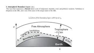
Understanding Temperature Structure and Cumulative Heating/Cooling in Atmospheric Boundary Layer
The temperature structure in the atmospheric boundary layer (ABL) is influenced by cumulative heating or cooling effects from the surface. During the day, heat accumulates within the ABL, while cooling occurs at night. The cumulative heating or cooling is more crucial for ABL evolution than instantaneous heat flux. Learn about nighttime cooling, daytime heating, and the idealized evolution of temperature profiles in the ABL.

Download Presentation

Please find below an Image/Link to download the presentation.
The content on the website is provided AS IS for your information and personal use only. It may not be sold, licensed, or shared on other websites without obtaining consent from the author. Download presentation by click this link. If you encounter any issues during the download, it is possible that the publisher has removed the file from their server.
E N D
Presentation Transcript
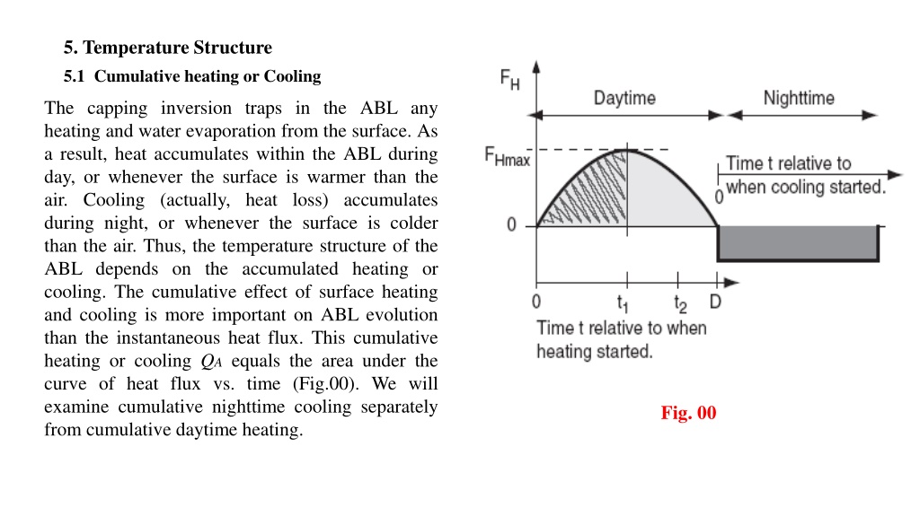
5. Temperature Structure 5.1 Cumulative heating or Cooling The capping inversion traps in the ABL any heating and water evaporation from the surface. As a result, heat accumulates within the ABL during day, or whenever the surface is warmer than the air. Cooling (actually, heat loss) accumulates during night, or whenever the surface is colder than the air. Thus, the temperature structure of the ABL depends on the accumulated heating or cooling. The cumulative effect of surface heating and cooling is more important on ABL evolution than the instantaneous heat flux. This cumulative heating or cooling QAequals the area under the curve of heat flux vs. time (Fig.00). We will examine cumulative nighttime cooling separately from cumulative daytime heating. Fig. 00
5.1.1 Nighttime During clear nights over land, heat flux from the air to the cold surface is relatively constant with time (dark shaded portion of Fig.10). If we define t as the time since cooling began, then the accumulated cooling per unit surface area is: For night, QA is a negative number because FH is negative for cooling. QA has units of J/m2. Dividing eq. (1a) by air density and specific heat ( air Cp) gives the kinematic form: Idealization of the heat flux curve over land during fair weather. Light shading shows total accumulated heating during the day, while the hatched region shows the portion of heating accumulated up to time t1 after heating started. Dark shading shows total accumulated cooling during the night. where QAk has units of K m. For a night with variable cloudiness that causes a variable surface heat flux.
5.1.2 Daytime On clear days, the nearly sinusoidal variation of solar elevation and downwelling solar radiation (Fig.2) causes nearly sinusoidal variation of surface net heat flux (Fig.3.). Let t be the time since FH becomes positive in the morning, D be the total duration of positive heat flux, and FH max be the peak value of heat flux (Fig. 1). These values can be found from data such as in Fig. 3. The accumulated daytime heating per unit surface area (units of J/m2) is: Fig 3: Typical diurnal variation of the surface heat budget. The F* net radiation curve comes from fig2. Fluxes are positive upward Fig 2 : Typical diurnal variation of radiative fluxes at the surface. Fluxes are positive upward.
Q) Use Fig. 3 to estimate the accumulated heating and cooling in kinematic form over the whole day and whole night.
6- Temperature-profile 6-1 Idealized Evolution A typical afternoon temperature profile is plotted in Fig. 4a. During the daytime, the environmental lapse rate in the mixed layer is nearly adiabatic. The unstable surface layer (plotted but not labeled in (Fig 5a) is in the bottom part of the mixed layer. Warm blobs of air called Thermalsrise from this surface layer up through the mixed layer, until they hit the temperature inversion in the entrainment zone. Fig. 5a shows a closer view of the surface layer (bottom 5 - 10% of ABL). These thermal circulations create strong turbulence, and cause pollutants, potential temperature, and moisture to be well mixed in the vertical (hence the name mixed layer). In the entrainment zone, free-atmosphere air is incorporated or entrained into the mixed layer, causing the mixed-layer depth to increase during the day. Pollutants trapped in the mixed layer cannot escape through the EZ, although cleaner, drier free atmosphere air is entrained into the mixed layer. Thus, the EZ is a one-way valve. Figure 4a Figure 5 a
At night, the bottom portion of the mixed layer becomes chilled by contact with the radiatively cooled ground. The bottom portion of this stable ABL is the surface layer sketched in Fig. 5b). Above the stable fig 4.b ABL is the residual layer. It has not felt the cooling from the ground, and hence retains the adiabatic lapse rate from the mixed layer of the previous day. Above that is the capping temperature inversion, which is the nonturbulent remnant entrainment zone. of the Figure 4 b Figure 5 b
During summer at mid- and high-latitudes, days are longer than nights during fair weather over land. More heating occurs during day than cooling at night. After a full 24 hours, the ending sounding is warmer than the starting sounding as illustrated in Fig.6 a & b. The convective mixed layer starts shallow in the morning, but rapidly grows through the residual layer. In the afternoon, it continues to rise slowly into the free atmosphere. If the air contains sufficient moisture, cumuliform clouds can exist. At night, cooling creates a shallow stable ABL near the ground, but leaves a thick residual layer in the middle of the ABL. Figure 6 a , b
During winter at mid- and high- Atitudes, more cooling occurs during the long nights than heating during the short days, in fair weather over land. Stable ABLs dominate, and there is net temperature decrease over 24 hours (Figs. 7 a,b). Any nonfrontal clouds present are typically stratiform or fog. Any residual layer that forms early in the night is quickly overwhelmed by the growing stable ABL. Figure 7 a , b
Fig. 8.a,b shows the corresponding structure of the ABL. Although both the mixed layer and residual layer have nearly adiabatic temperature profiles, the mixed layer is nonlocally unstable, while the residual layer is neutral. This difference causes pollutants to disperse at different rates in those two regions. Figure 8 a , b Daily evolution of boundary-layer structure by season, for fair weather over land. CI = Capping Inversion. Shading indicates static stability: white = unstable, light grey = neutral (as in the RL), darker greys indicate stronger static stability.


 Use Fig. 3 to estimate the accumulated heating and")