Using Excel Simulator in Teaching Macroeconomics: A Modern Approach
Explore the benefits of incorporating a macroeconomics simulator in teaching, focusing on addressing challenges in understanding model dynamics and how different models relate to each other. The simulator helps students grasp complex concepts such as shocks, policy responses, and real-world applications, enhancing their learning experience.
Download Presentation

Please find below an Image/Link to download the presentation.
The content on the website is provided AS IS for your information and personal use only. It may not be sold, licensed, or shared on other websites without obtaining consent from the author.If you encounter any issues during the download, it is possible that the publisher has removed the file from their server.
You are allowed to download the files provided on this website for personal or commercial use, subject to the condition that they are used lawfully. All files are the property of their respective owners.
The content on the website is provided AS IS for your information and personal use only. It may not be sold, licensed, or shared on other websites without obtaining consent from the author.
E N D
Presentation Transcript
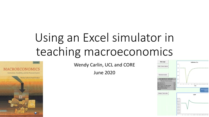
Using an Excel simulator in teaching macroeconomics Wendy Carlin, UCL and CORE June 2020
Why use a simulator in teaching macro? Modern macro teaches a purposeful policy maker(s) with objectives and constraints facing an economy subject to temporary and permanent supply and demand shocks Which courses? In the first year using CORE s The Economy, for example In the second year Intermediate macro using Carlin and Soskice or Blanchard, for example In the third year Topics in macroeconomic policy using Carlin and Soskice and papers / blogs such as Bank Underground and www.voxeu.org
Why use a simulator in teaching macro? The usual tools: equations, diagrams, data charts, historical and contemporary episodes of shocks and policy responses What students find hard: 1. understanding the model dynamics 2. how do the different models relate to each other? e.g. inflation-targeting monetary policy-maker with debt dynamics with exchange rate dynamics 3. relating the models to the world The macro simulator is invaluable for addressing (1) (3).
What students find hard: (1) understanding model dynamics Temporary positive AD shock
What students find hard: (2) how do the different models relate to each other? inflation-targeting monetary policy-maker with debt dynamics with exchange rate dynamics Small open economy with inflation-targeting CB; a negative permanent AD shock - what is the new medium-run equilibrium? - how does the economy adjust what does the CB do? - what role in adjustment is played by the forward-looking forex market? - what are the implications for public sector finances? Students have studied each model separately even good students would like to check their analytical treatment
Small open economy with inflation-targeting CB; a negative permanent AD shock
Small open economy with inflation-targeting CB; a negative permanent AD shock
Small open economy with inflation-targeting CB; a negative permanent AD shock
What students find hard: (3) relating the models to the world
How would this work in an online teaching environment? Very well perfect for individual or group online learning. You can ask them to compare analytical and simulation results and explain the dynamics They can plot the numerical results and compare to data You can add random shocks and ask them to collect the data and analyze it Get them to play the game (3 levels) where they are the macro policy maker faced by unpredictable shocks, which they have to diagnose and use policy tools to respond to Get them to write up their results very good for the difficult-to-teach dynamics of a deflation trap and hyperinflation
How would this work for research-based learning; for assessment? Opportunities for linking to research using theory data policy episodes Advanced students e.g. for dissertations can be set the challenge of creating a new simulator exercise related to a policy episode Assessment: for online open book assessment, simulator output can be required for validation of analytical solutions ----------------------------------
Mainstream macro model (Textbook: Carlin and Soskice, 2015) For the model, see textbook or https://discovery.ucl.ac.uk/id/eprint/16060/1/16060.pdf 3-equation model (IS/PC/MR) where the PC has backward-looking expectations; in the simulator, anchored expectations can be experimented with Open economy small open economy with inflation-targeting CB Open economy small open economy with fixed exchange rate (two versions in the simulator with and without an endogenous fiscal policy rule to stabilize inflation at the world inflation rate)
The structure of the 3-equation closed economy model CB minimizes its loss function, which expresses its objectives = + 2 2 T ( ) ( ) Min L y y t e t subject to the constraint from the supply side, in the Phillips curve = + E ( ) y y t t e which produces the monetary rule function that pins down the optimal output gap = T ( ) y y t e t which, is implemented in closed economy through choice of r using the IS equation (best-response Taylor Rule) y A ar y y a r r = = 1 t t ( ) 1 t e t S 16
3-equation open economy model: forward-looking CB and forex market (inflation shock) 17
Open economy with inflation targeting CB The CB s optimization problem: Real exchange rate: 2+ ? ?? ?? 2 Min ? = ?? ?? subject to ??= ?? 1+ ? ?? ?? ?? ?? = ?? ?? ??. In order to produce the desired output level, ?? , the CB chooses ?? 1 knowing the equations: ??= ? ??? 1+ ??? 1 and ?? ? = ??+1 ?? * P e P ; log Q q Q ? The forex market knows all of this too 18
Showing all the parameters of the open economy model in a diagram 19
Comparing an inflation shock in closed & open economies UCL ECON0016 TERM 2 LECTURE 3 20
Central bank reaction to a permanent negative demand shock 1. Find new MRE at Z 2. Output falls to B on new IS 3. Inflation falls to B on PC 4. CB & forex market calculate CB s optimal output gap on MR curve at C 5. RX shows how much r must be cut below r* : C on RX 6. IS shifts by equilibrium depreciation plus extra depreciation to take IS to C CB gradually raises r back to r*along RX (as expected) Since from C to Z, q appreciates as expected and IS moves to the left 7. * r r 8. 21
Simulator free online here https://global.oup.com/uk/orc/busecon/economics/carlin_soskice/student/excelsimulator/ Instructions on the website Examples on the website Try Question 1 https://global.oup.com/uk/orc/busecon/economics/carlin_soskice/studen t/excelsimulator/#Exercise1 UCL ECON0016 TERM 2 LECTURE 3 22
