Understanding Convolution in DT LTI Systems

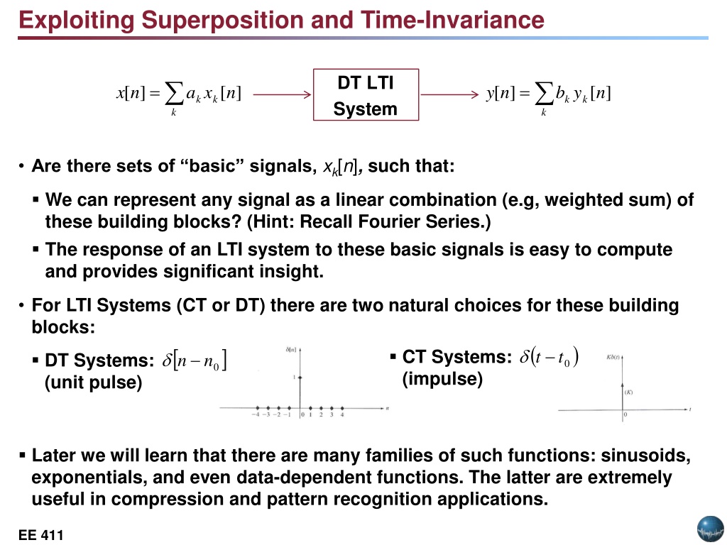
Exploiting Superposition and Time-Invariance DT LTI System k k = = [ ] [ ] [ ] [ ] x n a x n y n b y n k k k k Are there sets of basic signals, xk[n], such that: We can represent any signal as a linear combination (e.g, weighted sum) of these building blocks? (Hint: Recall Fourier Series.) The response of an LTI system to these basic signals is easy to compute and provides significant insight. For LTI Systems (CT or DT) there are two natural choices for these building blocks: n ( ) x.JPG t CT Systems: (impulse) 0t x.JPG DT Systems: (unit pulse) 0 n Later we will learn that there are many families of such functions: sinusoids, exponentials, and even data-dependent functions. The latter are extremely useful in compression and pattern recognition applications. EE 3512: Lecture 14, Slide 0 EE 411

Representation of DT Signals Using Unit Pulses EE 3512: Lecture 14, Slide 1 EE 411

Response of a DT LTI Systems Convolution DT LTI n h k k = = [ ] [ ] [ ] [ ] x n a x n y n b y n k k k k Define the unit pulse response, h[n], as the response of a DT LTI system to a unit pulse function, [n]. Using the principle of time-invariance: ] [ ] [ ] [ ] [ k n h k n n h n convolution operator Using the principle of linearity: = = = = = [ ] [ ] [ ] [ ] [ ] [ ] [ ] [ ] x n x k n k y n x k h n k x n h n k k Comments: convolution sum Recall that linearity implies the weighted sum of input signals will produce a similar weighted sum of output signals. Each unit pulse function, [n-k], produces a corresponding time-delayed version of the system impulse response function (h[n-k]). The summation is referred to as the convolution sum. The symbol * is used to denote the convolution operation. EE 3512: Lecture 14, Slide 2

LTI Systems and Impulse Response The output of any DT LTI is a convolution of the input signal with the unit pulse response: DT LTI n h = [ ] [ ] * [ ] y n x n h n [n x ] = = = = = [ ] [ ] [ ] [ ] [ ] [ ] [ ] [ ] x n x k n k y n x k h n k x n h n k k Any DT LTI system is completely characterized by its unit pulse response. Convolution has a simple graphical interpretation: EE 3512: Lecture 14, Slide 3 EE 411

Visualizing Convolution There are four basic steps to the calculation: The operation has a simple graphical interpretation: EE 3512: Lecture 14, Slide 4 EE 411

Calculating Successive Values We can calculate each output point by shifting the unit pulse response one sample at a time: = [ ] [ ] [ ] y n x k h n k = k y[n] = 0 for n < ??? y[-1] = y[0] = y[1] = y[n] = 0 for n > ??? Can we generalize this result? EE 3512: Lecture 14, Slide 5 EE 411

Graphical Convolution 2 1 (k ) h -1 -1 1 (k ) x -1 = k ) 3 = = ( ( ) ( 3 ) 0 y x k h k ( 3 ) h k = k ) 2 = = ( ( ) ( 2 ) 0 y x k h k ( 2 ) h k ) 1 = = ( 1 ( ) 1 )( 1 y ( 1 ) h k = + = ) 0 ( y 1 ( ) 0 )( 2 ( ) 1 )( 2 0 ( h ) k k = -6 -5 -4 -3 -2 -1 0 1 2 3 4 5 6 7 8 9 EE 3512: Lecture 14, Slide 6 EE 411

Graphical Convolution (Cont.) 2 1 (k ) h -1 -1 1 (k ) x -1 = ) 1 )( 1 + + ) 1 )( 1 = ) 1 ( y ( 2 ( ) 0 )( ( 2 1 ( h ) k = + ) 1 ) 2 ( y 1 ( + ) 0 )( 2 ( )( 2 ( h ) k ) 0 )( 1 + ) 1 )( 1 = ( ( 2 = + ) 3 ( y 1 ( + ) 0 )( 2 ( ) 0 )( + 3 ( h ) k ) 1 ) 0 )( 1 = ( 1 )( ( 1 = ) 1 = ) 4 ( y ( 1 )( 1 4 ( h ) k k = -6 -5 -4 -3 -2 -1 0 1 2 3 4 5 6 7 8 9 EE 3512: Lecture 14, Slide 7 EE 411

Graphical Convolution (Cont.) Observations: y[n] = 0 for n > 4 If we define the duration of h[n] as the difference in time from the first nonzero sample to the last nonzero sample, the duration of h[n], Lh, is 4 samples. Similarly, Lx = 3. The duration of y[n] is: Ly = Lx + Lh 1. This is a good sanity check. The fact that the output has a duration longer than the input indicates that convolution often acts like a low pass filter and smoothes the signal. EE 3512: Lecture 14, Slide 8 EE 411

Examples of DT Convolution Example: delayed unit-pulse Example: unit-pulse = = [ ] [ ] [ ] [ ] h n n n h n n 0 = = = = [ ] [ ] [ ] y n x k h n k [ ] [ ] [ ] y n x k h n k k k = = = = = = [ ] [ ] [ ] [ ] [ ] [ ] x k n k x n x k n n k x n n 0 0 k k Example: unit step Example: integration = ] [ u a n h = [ ] [ ] x n u n [ ] [ ] h n u n = n [ ] 1 n a = k = [ ] [ ] [ ] y n x k h n k k = [ ] [ ] [ ] y n x k h n k n = k = k = = [ ] [ ] [ ] x k u n k x k = k = n [ ] [ ] u n a u n = = + + n + ) 1 ( [ ] 1 ( ) [ ] 1 ... n a n = 1 a 0 + 1 1 n = 1 0 n a EE 3512: Lecture 14, Slide 9 EE 411

Properties of Convolution Implications Commutative: = [ ] * [ ] [ ] * [ ] x n h n h n x n Distributive: + = [ x ] * ( [ ] [ x ]) n x n h n h n 1 2 + ( [ ] * [ ]) ( [ ] * [ ]) n h n h n 1 2 Associative: = [ x ] * [ ] * [ h ] x n h n h n 1 h 2 = ( [ ] * [ ]) * [ ] n n n 1 2 ( [ ] * [ ]) * [ ] x n h n h n 2 1 EE 3512: Lecture 14, Slide 10 EE 411

Useful Properties of (DT) LTI Systems = Causality: [ ] 0 0 h n n = k Stability: h ] [ k Bounded Input Bounded Output Sufficient Condition: for [ ] x n x max = k = k = [ ] [ ] [ ] [ ] y n x k h n k x h n k max Necessary Condition: = k x = if [ ] h n k = = * Let [ ] [ / ] [ , ] then [ ] 1 (bounded) n h n h n x n = k = k = k = = = = * But y[0] [ ] 0 [ ] [ ] [ / ] [ ] [ ] x k h k h k h k h k h k EE 3512: Lecture 14, Slide 11 EE 411

Summary We introduced a method for computing the output of a discrete-time (DT) linear time-invariant (LTI) system known as convolution. We demonstrated how this operation can be performed analytically and graphically. We discussed three important properties: commutative, associative and distributive. Question: can we determine key properties of a system, such as causality and stability, by examining the system impulse response? There are several interactive tools available that demonstrate graphical convolution: ISIP: Convolution Java Applet. EE 3512: Lecture 14, Slide 12 EE 411