Discrete Optimization Methods Overview
Chapter 12
Discrete Optimization Methods
12.1 Solving by
Total Enumeration
•
If model has only a few discrete decision variables, the
most effective method of analysis is often the most
direct: enumeration of all the possibilities. [12.1]
•
Total enumeration solves a discrete optimization by
trying all possible combinations of discrete variable
values, computing for each the best corresponding
choice of any continuous variables. Among
combinations yielding a feasible solution, those with the
best objective function value are optimal. [12.2]
Swedish Steel Model
with All-or-Nothing Constraints
min 16
(75)y
1
+10
(250)y
2
+8 x
3
+9 x
4
+48 x
5
+60 x
6
+53 x
7
s.t.
75y
1
+
250y
2
+ x
3
+ x
4
+ x
5
+ x
6
+ x
7
= 1000
0
.
0
0
8
0
(
7
5
)
y
1
+
0
.
0
0
7
0
(
2
5
0
)
y
2
+
0
.
0
0
8
5
x
3
+
0
.
0
0
4
0
x
4
6
.
5
0
.
0
0
8
0
(
7
5
)
y
1
+
0
.
0
0
7
0
(
2
5
0
)
y
2
+
0
.
0
0
8
5
x
3
+
0
.
0
0
4
0
x
4
7
.
5
0
.
1
8
0
(
7
5
)
y
1
+
0
.
0
3
2
(
2
5
0
)
y
2
+
1
.
0
x
5
3
0
.
0
0
.
1
8
0
(
7
5
)
y
1
+
0
.
0
3
2
(
2
5
0
)
y
2
+
1
.
0
x
5
3
0
.
5
0
.
1
2
0
(
7
5
)
y
1
+
0
.
0
1
1
(
2
5
0
)
y
2
+
1
.
0
x
6
1
0
.
0
0
.
1
2
0
(
7
5
)
y
1
+
0
.
0
1
1
(
2
5
0
)
y
2
+
1
.
0
x
6
1
2
.
0
0
.
0
0
1
(
2
5
0
)
y
2
+
1
.
0
x
7
1
1
.
0
0
.
0
0
1
(
2
5
0
)
y
2
+
1
.
0
x
7
1
3
.
0
x
3
…
x
7
0
y
1
, y
2
= 0 or 1
(12.1)
Cost = 9967.06
y
1
* = 1, y
2
* = 0, x
3
* = 736.44, x
4
* = 160.06
x
5
* = 16.50, x
6
* = 1.00, x
7
* = 11.00
Swedish Steel Model
with All-or-Nothing Constraints
Exponential Growth
of Cases to Enumerate
•
Exponential growth makes total enumeration impractical
with models having more than a handful of discrete
decision variables. [12.3]
12.2 Relaxation of Discrete
Optimization Models
Example 12.1
Bison Booster
The Boosters are trying to decide what fundraising projects to
undertake at the next country fair. One option is customized T-
shirts, which will sell for $20 each; the other is sweatshirts selling for
$30. History shows that everything offered for sale will be sold
before the fair is over.
Materials to make the shirts are all donated by local
merchants, but the Boosters must rent the equipment for
customization. Different processes are involved, with the T-shirt
equipment renting at $550 for the period up to the fair, and the
sweatshirt equipment for $720. Display space presents another
consideration. The Boosters have only 300 square feet of display
wall area at the fair, and T-shirts will consume 1.5 square feet each,
sweatshirts 4 square feet each. What plan will net the most income?
Bison Booster Example Model
Net Income = 3450
x
1
* = 200, x
2
* = 0, y
1
* = 1, y
2
* = 0
(12.2)
Constraint Relaxation Scenarios
•
Double capacities
1.5x
1
+ 4x
2
600
x
1
400
y
1
x
2
150
y
2
x
1
, x
2
0
y
1
, y
2
= 0 or 1
•
Dropping first constraint
1.5x
1
+ 4x
2
300
x
1
200y
1
x
2
75y
2
x
1
, x
2
0
y
1
, y
2
= 0 or 1
Constraint Relaxation Scenarios
•
Treat discrete variables as continuous
1.5x
1
+ 4x
2
300
x
1
200y
1
x
2
75y
2
x
1
, x
2
0
0
y
1
1
0
y
2
1
Linear Programming Relaxations
•
Continuous relaxations
(
linear programming relaxations
if
the given model is an ILP) are formed by treating any
discrete variables as continuous while retaining all other
constraints. [12.6]
•
LP relaxations of ILPs are by far the most used relaxation
forms because they bring all the power of LP to bear on
analysis of the given discrete models. [12.7]
Proving Infeasibility with Relaxations
•
If a constraint relaxation is infeasible, so is the full model it
relaxes. [12.8]
Solution Value Bounds from
Relaxations
•
The optimal value of any
relaxation of a maximize model
yields an upper bound on the
optimal value of the full model.
The optimal value of any
relaxation of a minimize model
yields an lower bound. [12.9]
Feasible solutions in
relaxation
Feasible solutions
in true model
True optimum
Example 11.3
EMS Location Planning
Minimum Cover EMS Model
(12.3)
x
2
1
x
1
+ x
2
1
x
1
+ x
3
1
x
3
1
x
3
1
x
2
1
x
2
+ x
4
1
x
3
+ x
4
1
x
8
1
x
i
= 0 or 1
j=1,…,10
x
4
+ x
6
1
x
4
+ x
5
1
x
4
+ x
5
+ x
6
1
x
4
+ x
5
+ x
7
1
x
8
+ x
9
1
x
6
+ x
9
1
x
5
+ x
6
1
x
5
+ x
7
+ x
10
1
x
8
+ x
9
1
x
9
+ x
10
1
x
10
1
x
2
* = x
3
* = x
4
* = x
6
*
= x
8
* = x
10
* =1,
x
1
* = x
5
* = x
7
* = x
9
*
= 0
Minimum Cover EMS Model
with Relaxation
(12.4)
x
2
1
x
1
+ x
2
1
x
1
+ x
3
1
x
3
1
x
3
1
x
2
1
x
2
+ x
4
1
x
3
+ x
4
1
x
8
1
0
x
j
1
j=1,…,10
x
4
+ x
6
1
x
4
+ x
5
1
x
4
+ x
5
+ x
6
1
x
4
+ x
5
+ x
7
1
x
8
+ x
9
1
x
6
+ x
9
1
x
5
+ x
6
1
x
5
+ x
7
+ x
10
1
x
8
+ x
9
1
x
9
+ x
10
1
x
10
1
Optimal Solutions from Relaxations
•
If an optimal solution to a constraint relaxation is also
feasible in the model it relaxes, the solution is optimal in that
original model. [12.10]
Rounded Solutions from Relaxations
•
Many relaxations produce optimal solutions that are easily
“rounded” to good feasible solutions for the full model.
[12.11]
•
The objective function value of any (integer) feasible
solution to a maximizing discrete optimization problem
provides a lower bound on the integer optimal value, and
any (integer) feasible solution to a minimizing discrete
optimization problem provides an upper bound. [12.12]
Rounded Solutions from Relaxation:
EMS Model
(12.5)
12.3 Stronger LP Relaxations,
Valid Inequalities,
and Lagrangian Relaxation
•
A relaxation is
strong
or
sharp
if its optimal value
closely bounds that of the true model, and its optimal
solution closely approximates an optimum in the full
model. [12.13]
•
Equally correct ILP formulations of a discrete problem
may have dramatically different LP relaxation optima.
[12.14]
Choosing Big-M Constants
•
Whenever a discrete model requires sufficiently large
big-M’s, the strongest relaxation will result from models
employing the smallest valid choice of those
constraints. [12.15]
Bison Booster Example Model
with Relaxation in Big-M Constants
•
Max 20x
1
+ 30x
2
– 550y
1
– 720y
2
(Net income)
s.t.
1.5x
1
+ 4x
2
300
(Display space)
x
1
200y
1
(T-shirt if equipment)
x
2
75y
2
(Sweatshirt if equipment)
x
1
, x
2
0
y
1
, y
2
= 0 or 1
•
Max 20x
1
+ 30x
2
– 550y
1
– 720y
2
(Net income)
s.t.
1.5x
1
+ 4x
2
300
(Display space)
x
1
10000y
1
(T-shirt if equipment)
x
2
10000y
2
(Sweatshirt if equipment)
x
1
, x
2
0
y
1
, y
2
= 0 or 1
Net Income = 3450
x
1
* = 200, x
2
* = 0, y
1
* = 1, y
2
* = 0
(12.2)
(12.6)
Valid Inequalities
•
A linear inequality is a
valid inequality
for a given
discrete optimization model if it holds for all (integer)
feasible solutions to the model. [12.16]
•
To strengthen a relaxation, a valid inequality must cut
off (render infeasible) some feasible solutions to the
current LP relaxation that are not feasible in the full ILP
model. [12.17]
Example 11.10
Tmark Facilities Location
Example 11.10
Tmark Facilities Location
Tmark Facilities Location Example
with LP Relaxation
(12.8)
s.t.
y
4
*=y
8
*= 1
y
1
*=y
2
*= y
3
*=y
5
*= y
6
*=y
7
*= 0
Total Cost = 10153
Tmark Facilities Location Example
with LP Relaxation
(12.8)
s.t.
Lagrangian Relaxations
Example 11.6
CDOT Generalized Assignment
The Canadian Department of Transportation encountered a problem
of the generalized assignment form when reviewing their allocation of coast
guard ships on Canada’s Pacific coast. The ships maintain such
navigational aids as lighthouses and buoys. Each of the districts along the
coast is assigned to one of a smaller number of coast guard ships. Since
the ships have different home bases and different equipment and operating
costs, the time and cost for assigning any district varies considerably among
the ships. The task is to find a minimum cost assignment.
Table 11.6 shows data for our (fictitious) version of the problem.
Three ships-the Estevan, the Mackenzie, and the Skidegate--are available to
serve 6 districts. Entries in the table show the number of weeks each ship
would require to maintain aides in each district, together with the annual cost
(in thousands of Canadian dollars). Each ship is available SG weeks per
year.
Example 11.6
CDOT Generalized Assignment
CDOT Assignment Model
min 130x
1,1
+460x
1,2
+40x
1,3
+30x
2,1
+150x
2,2
+370x
2,3
+510x
3,1
+20x
3,2
+120x
3,3
+30x
4,1
+40x
4,2
+390x
4,3
+340x
5,1
+30x
5,2
+40x
5,3
+20x
6,1
+450x
6,2
+30x
6,3
s.t.
(12.12)
x
1,1
+ x
1,2
+ x
1,3
=
1
x
2,1
+ x
2,2
+ x
2,3
=
1
x
3,1
+ x
3,2
+ x
3,3
=
1
x
4,1
+ x
4,2
+ x
4,3
=
1
x
5,1
+ x
5,2
+ x
5,3
=
1
x
6,1
+ x
6,2
+ x
6,3
=
1
X
i,j
= 0 or 1
i=1,…,6; j=1,…,3
x
1,1
*=x
4,1
*=x
6,1
*=x
2,2
*=
x
5,2
*=x
3,3
*=1
Total Cost = 480
30x
1,1
+ 50x
2,1
+ 10x
3,1
+ 11x
4,1
+ 13x
5,1
+ 9x
6,1
50
10x
1,2
+ 20x
2,2
+ 60x
3,2
+ 10x
4,2
+ 10x
5,2
+ 17x
6,2
50
70x
1,3
+ 10x
2,3
+ 10x
3,3
+ 15x
4,3
+ 8x
5,3
+ 12x
6,3
50
Largrangian Relaxation of the
CDOT Assignment Example
(12.13)
X
i,j
= 0 or 1
i=1,…,6; j=1,…,3
30x
1,1
+ 50x
2,1
+ 10x
3,1
+ 11x
4,1
+ 13x
5,1
+ 9x
6,1
50
10x
1,2
+ 20x
2,2
+ 60x
3,2
+ 10x
4,2
+ 10x
5,2
+ 17x
6,2
50
70x
1,3
+ 10x
2,3
+ 10x
3,3
+ 15x
4,3
+ 8x
5,3
+ 12x
6,3
50
More on Lagrangian Relaxations
Largrangian Relaxation of the
CDOT Assignment Example
(12.13)
X
i,j
= 0 or 1
i=1,…,6; j=1,…,3
30x
1,1
+ 50x
2,1
+ 10x
3,1
+ 11x
4,1
+ 13x
5,1
+ 9x
6,1
50
10x
1,2
+ 20x
2,2
+ 60x
3,2
+ 10x
4,2
+ 10x
5,2
+ 17x
6,2
50
70x
1,3
+ 10x
2,3
+ 10x
3,3
+ 15x
4,3
+ 8x
5,3
+ 12x
6,3
50
12.4 Branch and Bound Search
•
Branch and bound algorithms combine a subset
enumeration strategy with the relaxation methods.
They systematically form classes of solutions and
investigate whether the classes can contain optimal
solutions by analyzing associated relaxations.
Example 12.2
River Power
River Power has 4 generators currently available for production
and wishes to decide which to put on line to meet the expected 700-
MW peak demand over the next several hours. The following table
shows the cost to operate each generator (in $1000/hr) and their
outputs (in MW). Units must be completely on or completely off.
Example 12.2
River Power
x
1
* = x
3
* = 1
Cost = 12
Branch and Bound Search:
Definitions
•
A
partial solution
has some decision variables fixed,
with others left
free
or undetermined. We denote free
components of a partial solution by the symbol #.
[12.22]
•
The completions of a partial solution to a given model
are the possible full solutions agreeing with the partial
solution on all fixed components. [12.23]
Tree Search
•
B
r
a
n
c
h
a
n
d
b
o
u
n
d
s
e
a
r
c
h
b
e
g
i
n
s
a
t
i
n
i
t
i
a
l
o
r
r
o
o
t
s
o
l
u
t
i
o
n
x
(
0
)
=
(
#
,
…
,
#
)
w
i
t
h
a
l
l
v
a
r
i
a
b
l
e
s
f
r
e
e
.
[
1
2
.
2
4
]
•
Branch and
bound searches terminate or fathom a
partial
solution when they either identify a best completion or prove
that none can produce an optimal solution in the overall
model. [12.25]
•
When a partial solution cannot be terminated in a branch-
and-bound search of a 0-1 discrete optimization model, it is
branched by creating a 2 subsidiary partial solutions derived
by fixing a previously free binary variable. One of these
partial solutions matches the current except that the variable
chosen is fixed =1, and the other =0. [12.26]
Tree Search
•
Branch and bound search stops when every partial solution
in the tree has been either branched or terminated. [12.27]
•
Depth first search selects at each iteration an active partial
solution with the most components fixed (i.e., one deepest in
the search tree). [12.28]
LP-Based Branch and Bound Solution
of the River Power Example
X
4
=1
X
4
=0
1
2
3
X
2
=1
X
2
=0
X
3
=1
X
3
=0
4
5
6
X
1
=1
X
1
=0
7
X
3
=1
X
3
=0
8
9
10
Incumbent Solutions
Candidate Problems
•
The
candidate problem
associated with any partial solution
to an optimization model is the restricted version of the
model obtained when variables are fixed as in the partial
solution.
[12.31]
•
The feasible completions of any partial solution are exactly
the feasible solutions to the corresponding candidate
problem, and thus the objective value of the best feasible
completion is the optimal objective value of the candidate
problem. [12.32]
Terminating Partial Solutions with
Relaxations
•
If any relaxation of a
candidate problem proves infeasible,
the
associated partial solution can be terminated because it
has no feasible completions.
[12.33]
•
If any relaxation of a
candidate problem has optimal objective
value no better than the current incumbent solution value, the
associated partial solution can be terminated because no
feasible completion can improve on the incumbent.
[12.34]
•
If an optimal solution to any constraint relaxation of a
candidate problem is feasible in the full candidate, it is a best
feasible completion of the associated partial solution. After
checking whether a new incumbent has been discovered, the
partial solution can be terminated.
[12.35]
Algorithm 12A:
LP-Based Branch and Bound (0-1 ILPs)
Algorithm 12A:
LP-Based Branch and Bound (0-1 ILPs)
Algorithm 12A:
LP-Based Branch and Bound (0-1 ILPs)
Branching Rules for
LP-Based Branch and Bound
•
LP-based branch and bound algorithms always branch by
fixing an integer-restricted decision variable that had a
fractional value in the associated candidate problem
relaxation. [12.36]
•
When more than one integer-restricted variable is fractional
in the relaxation optimum, LP-based branch and bound
algorithms often branch by fixing the one closest to an
integer value. [12.37]
•
Tie-breaker
LP-Based Branch and Bound Solution
of the River Power Example
x
1
* = x
3
* = 1
Cost = 12
LP-Based Branch and Bound Solution
of the River Power Example
X
4
=1
X
4
=0
1
2
3
X
2
=1
X
2
=0
X
3
=1
X
3
=0
4
5
6
X
1
=1
X
1
=0
7
X
3
=1
X
3
=0
8
9
10
12.5 Rounding, Parent Bounds,
Enumerations Sequences, and
Stopping Early in Branch and Bound
•
Refinements of Branch and bound algorithms.
NASA Example Model
max 200x
1
+3x
2
+20x
3
+50x
4
+70x
5
+20 x
6
+5x
7
+10x
8
+200x
9
+150x
10
+18x
11
+8x
12
+300x
13
+185x
14
s.t. 6x
1
+ 2x
2
+ 3x
3
+ 1x
7
+ 4x
9
+ 5x
12
10
3x
2
+ 5x
3
+ 5x
5
+ 8x
7
+ 5x
9
+ 8x
10
+ 7x
12
+ 1x
13
+ 4x
14
12
8x
5
+ 1x
6
+ 4x
10
+ 2x
11
+ 4x
13
+ 5x
14
14
8x
6
+ 5x
8
+ 7x
11
+ 1x
13
+ 3x
14
14
10x
4
+ 4x
6
+ 1x
13
+ 3x
14
14
x
4
+ x
5
1
x
8
+ x
11
1
x
9
+ x
14
1
x
i
= 0 or 1
j=1,…,14
(12.16)
x
11
x
2
x
4
x
3
x
5
x
3
x
6
x
3
x
7
x
3
x
1
* = x
3
* = x
4
* = x
8
*
= x
13
* = x
14
* =1
Value = 765
Rounding for Incumbent Solutions
•
If convenient rounding schemes are available, the relaxation
optimum for every partial solution that cannot be terminated
in a branch and bound search is usually rounded to a
feasible solution for the full model prior to branching. The
feasible solution provides a new incumbent if it is better than
any known. [12.38]
Branch and Bound Family Tree
Terminology
•
Any node created directly from another by branching is called
a
child
, and the branched node is its
parent
.
•
The relaxation optimal value for the parent of any partial
solution to a minimize model provides a lower bound on the
objective value of any completion of its children. The
relaxation optimal value for the parent in a maximize model
provides an upper bound. [12.39]
•
Whenever a branch and bound search discovers a new
incumbent solution, any active partial solution with parent
bound no better than the new incumbent solution value can
immediately be terminated. [12.40]
Bounds on the Error of Stopping
with the Incumbent Solution
•
The least relaxation optimal value for parents of the active
partial solutions in a minimizing branch and bound search
always provides a lower bound on the optimal solution value
of the full model. The greatest relaxation optimal value for
parents in a maximizing search provides an upper bound.
[12.41]
•
At any stage of a branch and bound search, the difference
between the incumbent solution value and the best parent
bound of any active partial solution shows the maximum error
in accepting the incumbent as an approximate optimum.
[12.42]
Depth First, Best First, and Depth
Forward Best Back Sequences
•
Best first
search selects at each iteration an active partial
solution with best parent bound. [12.43]
•
Depth forward best back
search selects a deepest active
partial solution after branching a node, but one with best
parent bound after a termination. [12.44]
•
When several active partial solutions tie for deepest or best
parent bound, the nearest child chooses the one with last
fixed variable value nearest the corresponding component of
the parent LP relaxation. [12.45]
Branch and Cut Search
•
Branch and cut
algorithms modify the basic branch and
bound strategy of Algorithm 12A by attempting to strengthen
relaxations with new inequalities before branching a partial
solution. Added constraints should hold for all feasible
solutions to the full discrete model, but they should cut off
(render infeasible) the last relaxation optimum. [12.46]
Algorithm 12B:
Branch and Cut (0-1 ILPs)
Algorithm 12B:
Branch and Cut (0-1 ILPs)
Algorithm 12B:
Branch and Cut (0-1 ILPs)
12.6 Improving Search Heuristics
for Discrete Optimization INLPS
•
Many large combinatorial optimization models,
especially INLPs with nonlinear objective functions, are
too large for enumeration and lack strong relaxations
that are tractable.
•
D
i
s
c
r
e
t
e
N
e
i
g
h
b
o
r
h
o
o
d
s
a
n
d
M
o
v
e
S
e
t
s
:
I
m
p
r
o
v
i
n
g
s
e
a
r
c
h
e
s
o
v
e
r
d
i
s
c
r
e
t
e
v
a
r
i
a
b
l
e
s
d
e
f
i
n
e
n
e
i
g
h
b
o
r
h
o
o
d
s
b
y
s
p
e
c
i
f
y
i
n
g
a
m
o
v
e
s
e
t
M
o
f
m
o
v
e
s
a
l
l
o
w
e
d
.
T
h
e
c
u
r
r
e
n
t
s
o
l
u
t
i
o
n
a
n
d
a
l
l
r
e
a
c
h
a
b
l
e
f
r
o
m
i
t
i
n
a
s
i
n
g
l
e
m
o
v
e
x
M
c
o
m
p
r
i
s
e
i
t
s
n
e
i
g
h
b
o
r
h
o
o
d
.
[
1
2
.
4
7
]
Algorithm 12C: Rudimentary
Improving Search Algorithm
S
t
e
p
0
:
I
n
i
t
i
a
l
i
z
a
t
i
o
n
.
C
h
o
o
s
e
a
n
y
s
t
a
r
t
i
n
g
f
e
a
s
i
b
l
e
s
o
l
u
t
i
o
n
x
(
0
)
,
a
n
d
s
e
t
s
o
l
u
t
i
o
n
i
n
d
e
x
t
0
.
S
t
e
p
1
:
L
o
c
a
l
O
p
t
i
m
u
m
.
I
f
n
o
m
o
v
e
x
i
n
m
o
v
e
s
e
t
M
i
s
b
o
t
h
i
m
p
r
o
v
i
n
g
a
n
d
f
e
a
s
i
b
l
e
a
t
c
u
r
r
e
n
t
s
o
l
u
t
i
o
n
x
(
t
)
,
s
t
o
p
.
P
o
i
n
t
x
(
t
)
i
s
a
l
o
c
a
l
o
p
t
i
m
u
m
.
S
t
e
p
2
:
M
o
v
e
.
C
h
o
o
s
e
s
o
m
e
i
m
p
r
o
v
i
n
g
f
e
a
s
i
b
l
e
m
o
v
e
x
M
a
s
x
(
t
+
1
)
.
S
t
e
p
3
:
S
t
e
p
.
U
p
d
a
t
e
x
(
t
+
1
)
x
(
t
)
+
x
(
t
+
1
)
.
S
t
e
p
4
:
I
n
c
r
e
m
e
n
t
.
I
n
c
r
e
m
e
n
t
t
t
+
1
,
a
n
d
r
e
t
u
r
n
t
o
S
t
e
p
1
.
Example 11.8
NCB Circuit Board TSP
Figure 11.4 shows the tiny example that we will investigate for
fictional board manufacturer NCB. We seek an optimal route through the 10
hole locations indicated. Table 11.7 reports straight-line distances d
i,j
between hole locations i and j. Lines in Figure 11.4 show a fair quality
solution with total length 92.8 inches. The best route is 11 inches shorter
(see Section 12.6).
Quadratic Assignment Formulation
of the TSP
(12.20)
s.t.
Let
Choosing a Move Set
•
The move set
M
of a discrete improving search must be
compact enough to be checked at each iteration for
improving feasible neighbors. [12.48]
•
The solution produced by a discrete improving search
depends on the move set (or neighborhood) employed, with
larger move sets generally resulting in superior local optima.
[12.49]
Multistart Search
•
Multistart
or keeping the best of several local optima
obtained by searches from different starting solutions is one
way to improve the heuristic solutions produced by
improving search. [12.50]
12.7 Tabu, Simulated Annealing, and
Genetic Algorithm Extensions of
Improving Search
Difficulty with Allowing Nonimproving Moves
•
Nonimproving moves will lead to infinite cycling of
improving search unless some provision is added to
prevent repeating solutions. [12.51]
Tabu Search
•
Tabu search deals with cycling by temporarily
forbidding moves that would return to a solution
recently visited. [12.52]
Algorithm 12D: Tabu Search
Algorithm 12D: Tabu Search
S
t
e
p
5
:
T
a
b
u
L
i
s
t
.
R
e
m
o
v
e
f
r
o
m
t
h
e
l
i
s
t
o
f
t
a
b
u
o
f
f
o
r
b
i
d
d
e
n
m
o
v
e
s
a
n
y
t
h
a
t
h
a
v
e
b
e
e
n
o
n
i
t
f
o
r
a
s
u
f
f
i
c
i
e
n
t
n
u
m
b
e
r
o
f
i
t
e
r
a
t
i
o
n
s
,
a
n
d
a
d
d
a
c
o
l
l
e
c
t
i
o
n
o
f
m
o
v
e
s
t
h
a
t
i
n
c
l
u
d
e
s
a
n
y
r
e
t
u
r
n
i
n
g
i
m
m
e
d
i
a
t
e
l
y
f
r
o
m
x
(
t
+
1
)
t
o
x
(
t
)
.
S
t
e
p
6
:
I
n
c
r
e
m
e
n
t
.
I
n
c
r
e
m
e
n
t
t
t
+
1
,
a
n
d
r
e
t
u
r
n
t
o
S
t
e
p
1
.
Simulated Annealing Search
•
Simulated annealing
algorithms control cycling by
accepting non-improving moves according to
probabilities tested with computer-generated random
numbers. [12.53]
•
The move selection process at each iteration begins
with random choice of a provisional feasible move,
totally ignoring its objective function impact. Next, the
net objective function improvement
obj is computed
for the chosen move. The move is always accepted if it
improves (obj > 0), and otherwise
probability of acceptance = e
obj/q
where q=temp.
Algorithm 12E:
Simulated Annealing Search
Algorithm 12E:
Simulated Annealing Search
Genetic Algorithms
•
Genetic
algorithms evolve good heuristic optima by
operations combining members of an improving
population
of individual solutions. [12.54]
•
Crossover combines a pair of “parent” solutions to
produce a pair of :children” by breaking both parent
vectors at the same point and reassembling the first
part of one parent solution with the second part of the
other, and vice versa. [12.55]
Genetic Algorithms
•
T
h
e
e
l
i
t
e
s
t
s
t
r
a
t
e
g
y
f
o
r
i
m
p
l
e
m
e
n
t
a
t
i
o
n
o
f
g
e
n
e
t
i
c
a
l
g
o
r
i
t
h
m
s
f
o
r
m
s
e
a
c
h
n
e
w
g
e
n
e
r
a
t
i
o
n
a
s
a
m
i
x
t
u
r
e
o
f
e
l
i
t
e
(
b
e
s
t
)
s
o
l
u
t
i
o
n
s
h
e
l
d
o
v
e
r
f
r
o
m
t
h
e
p
r
e
v
i
o
u
s
g
e
n
e
r
a
t
i
o
n
,
i
m
m
i
g
r
a
n
t
s
o
l
u
t
i
o
n
s
a
d
d
e
d
a
r
b
i
t
r
a
r
i
l
y
t
o
i
n
c
r
e
a
s
e
d
i
v
e
r
s
i
t
y
,
a
n
d
c
h
i
l
d
r
e
n
o
f
c
r
o
s
s
o
v
e
r
o
p
e
r
a
t
i
o
n
s
o
n
n
o
n
-
o
v
e
r
l
a
p
p
i
n
g
p
a
i
r
s
o
f
s
o
l
u
t
i
o
n
s
i
n
t
h
e
p
r
e
v
i
o
u
s
p
o
p
u
l
a
t
i
o
n
.
[
1
2
.
5
6
]
•
Effective genetic algorithm search requires a choice for
encoding problem solutions that often, if not always,
preserves solution feasibility after crossover. [12.57]
Algorithm 12F:
Genetic Algorithm Search
S
t
e
p
0
:
I
n
i
t
i
a
l
i
z
a
t
i
o
n
.
C
h
o
o
s
e
a
p
o
p
u
l
a
t
i
o
n
s
i
z
e
p
,
i
n
i
t
i
a
l
s
t
a
r
t
i
n
g
f
e
a
s
i
b
l
e
s
o
l
u
t
i
o
n
s
x
(
1
)
,
…
,
x
(
p
)
,
a
n
g
e
n
e
r
a
t
i
o
n
l
i
m
i
t
t
m
a
x
,
a
n
d
a
p
o
p
u
l
a
t
i
o
n
s
u
b
d
i
v
i
s
i
o
n
s
p
e
f
o
r
e
l
i
t
e
s
,
p
i
f
o
r
i
m
m
i
g
r
a
n
t
s
,
a
n
d
p
c
f
o
r
c
r
o
s
s
o
v
e
r
s
.
A
l
s
o
s
e
t
t
h
e
g
e
n
e
r
a
t
i
o
n
i
n
d
e
x
t
0
.
S
t
e
p
1
:
S
t
o
p
p
i
n
g
.
I
f
t
=
t
m
a
x
,
s
t
o
p
a
n
d
r
e
p
o
r
t
t
h
e
b
e
s
t
s
o
l
u
t
i
o
n
o
f
t
h
e
c
u
r
r
e
n
t
p
o
p
u
l
a
t
i
o
n
a
s
a
n
a
p
p
r
o
x
i
m
a
t
e
o
p
t
i
m
u
m
.
S
t
e
p
2
:
E
l
i
t
e
.
I
n
i
t
i
a
l
i
z
e
t
h
e
p
o
p
u
l
a
t
i
o
n
o
f
g
e
n
e
r
a
t
i
o
n
t
+
1
w
i
t
h
c
opies of the p
e
best solutions in the current generation.
S
t
e
p
3
:
I
m
m
i
g
r
a
n
t
s
.
A
r
b
i
t
r
a
r
i
l
y
c
h
o
o
s
e
p
i
n
e
w
i
m
m
i
g
r
a
n
t
f
e
a
s
i
b
l
e
s
o
l
u
t
i
o
n
s
,
a
n
d
i
n
c
l
u
d
e
t
h
e
m
i
n
t
h
e
t
+
1
p
o
p
u
l
a
t
i
o
n
.
Algorithm 12F:
Genetic Algorithm Search
S
t
e
p
4
:
C
r
o
s
s
o
v
e
r
.
C
h
o
o
s
e
p
c
/
2
n
o
n
-
o
v
e
r
l
a
p
p
i
n
g
p
a
i
r
s
o
f
s
o
l
u
t
i
o
n
s
f
r
o
m
t
h
e
g
e
n
e
r
a
t
i
o
n
t
p
o
p
u
l
a
t
i
o
n
,
a
n
d
e
x
e
c
u
t
e
c
r
o
s
s
o
v
e
r
o
n
e
a
c
h
p
a
i
r
a
t
a
n
i
n
d
e
p
e
n
d
e
n
t
l
y
c
h
o
s
e
n
r
a
n
d
o
m
c
u
t
p
o
i
n
t
t
o
c
o
m
p
l
e
t
e
t
h
e
g
e
n
e
r
a
t
i
o
n
t
+
1
p
o
p
u
l
a
t
i
o
n
.
S
t
e
p
5
:
I
n
c
r
e
m
e
n
t
.
I
n
c
r
e
m
e
n
t
t
t
+
1
,
a
n
d
r
e
t
u
r
n
t
o
S
t
e
p
1
.
12.8 Constructive Heuristics
•
Improving search heuristics in Section 12.6 and 12.7
move from complete solution to complete solution.
•
The constructive search alternative follows a strategy
more like the branch and bound searches proceeding
through partial solutions, choosing values for decision
variables one at a time and (often) stopping upon
completion of a first feasible solution.
Algorithm 12G:
Rudimentary Constructive Search
Greedy Choices of Variables to Fix
•
Greedy constructive heuristics elect the next variable to fix
and its value that does least damage to feasibility and most
helps the objective function, based on what has already
been fixed in the current partial solution. [12.58]
•
In large, especially non-linear, discrete models, or when
time is limited, constructive search is often the only effective
optimization-based approach to finding good solutions.
[12.59]
Discrete optimization methods, such as total enumeration and constraint relaxations, are valuable techniques for solving problems with discrete decision variables. Total enumeration involves exhaustively trying all possibilities to find optimal solutions, while constraint relaxations offer a more tractable approach. Exponential growth can make total enumeration impractical for models with many variables. An example involving fundraising projects illustrates the application of these methods in real-world scenarios.

Download Presentation

Please find below an Image/Link to download the presentation.
The content on the website is provided AS IS for your information and personal use only. It may not be sold, licensed, or shared on other websites without obtaining consent from the author.If you encounter any issues during the download, it is possible that the publisher has removed the file from their server.
You are allowed to download the files provided on this website for personal or commercial use, subject to the condition that they are used lawfully. All files are the property of their respective owners.
The content on the website is provided AS IS for your information and personal use only. It may not be sold, licensed, or shared on other websites without obtaining consent from the author.
E N D
Presentation Transcript
Chapter 12 Discrete Optimization Methods
12.1 Solving by Total Enumeration If model has only a few discrete decision variables, the most effective method of analysis is often the most direct: enumeration of all the possibilities. [12.1] Total enumeration solves a discrete optimization by trying all possible combinations of discrete variable values, computing for each the best corresponding choice of any continuous variables. Among combinations yielding a feasible solution, those with the best objective function value are optimal. [12.2]
Swedish Steel Model with All-or-Nothing Constraints min 16(75)y1+10(250)y2 +8 x3+9 x4+48 x5+60 x6 +53 x7 s.t. 75y1+ 250y2+ x3+ x4+ x5+ x6 + x7 = 1000 0.0080(75)y1+ 0.0070(250)y2+0.0085x3+0.0040x4 0.0080(75)y1+ 0.0070(250)y2+0.0085x3+0.0040x4 0.180(75)y1+ 0.032(250)y2+ 1.0 x5 0.180(75)y1+ 0.032(250)y2+ 1.0 x5 0.120(75)y1+ 0.011(250)y2+ 1.0 x6 0.120(75)y1+ 0.011(250)y2+ 1.0 x6 0.001(250)y2+ 1.0 x7 0.001(250)y2+ 1.0 x7 x3 x7 0 y1, y2= 0 or 1 y1* = 1, y2* = 0, x3* = 736.44, x4* = 160.06 x5* = 16.50, x6* = 1.00, x7* = 11.00 (12.1) 6.5 7.5 30.0 30.5 10.0 12.0 11.0 13.0 Cost = 9967.06
Swedish Steel Model with All-or-Nothing Constraints Discrete Combination y1 0 0 1 1 Corresponding Continuous Solution Objective Value y2 0 1 0 1 x3 x4 x5 x6 x7 823.11 646.67 736.44 561.56 125.89 63.33 160.06 94.19 30.00 22.00 16.50 8.50 10.00 7.25 1.00 0.00 11.00 10.75 11.00 10.75 10340.89 10304.08 9967.06 10017.94
Exponential Growth of Cases to Enumerate Exponential growth makes total enumeration impractical with models having more than a handful of discrete decision variables. [12.3]
12.2 Relaxation of Discrete Optimization Models Constraint Relaxations Model ( ?) is a constraint relaxations of model (P) if every feasible solution to (P) is also feasible in ( ?) and both models have the same objective function. [12.4] Relaxation should be significantly more tractable than the models they relax, so that deeper analysis is practical. [12.5]
Example 12.1 Bison Booster The Boosters are trying to decide what fundraising projects to undertake at the next country fair. One option is customized T- shirts, which will sell for $20 each; the other is sweatshirts selling for $30. History shows that everything offered for sale will be sold before the fair is over. Materials to make the shirts are all donated by local merchants, but the Boosters must rent the equipment for customization. Different processes are involved, with the T-shirt equipment renting at $550 for the period up to the fair, and the sweatshirt equipment for $720. Display space presents another consideration. The Boosters have only 300 square feet of display wall area at the fair, and T-shirts will consume 1.5 square feet each, sweatshirts 4 square feet each. What plan will net the most income?
Bison Booster Example Model Decision variables: x1 number of T-shirts made and sold x2 number of sweatshirts made and sold y1 1 if T-shirt equipment is rented; =0 otherwise y1 1 if sweatshirt equipment is rented; =0 otherwise Max 20x1 + 30x2 550y1 720y2 (Net income) s.t. 1.5x1 + 4x2 300 x1 200y1 x2 75y2 x1, x2 0 y1, y2 = 0 or 1 x1* = 200, x2* = 0, y1* = 1, y2* = 0 (Display space) (T-shirt if equipment) (Sweatshirt if equipment) (12.2) Net Income = 3450
Constraint Relaxation Scenarios Double capacities 1.5x1 + 4x2 600 x1 400y1 x2 150y2 x1, x2 0 y1, y2 = 0 or 1 Dropping first constraint 1.5x1+ 4x2 300 x1 200y1 x2 75y2 x1, x2 0 y1, y2 = 0 or 1 Net Income = 7450 ?1* = 400, ?2* = 0, ?1* = 1, ?2 * = 0 Net Income = 4980 ?1* = 200, ?2* = 75, ?1* = 1, ?2 * = 1
Constraint Relaxation Scenarios Treat discrete variables as continuous 1.5x1 + 4x2 300 x1 200y1 x2 75y2 x1, x2 0 0 y1 1 0 y2 1 Net Income = 3450 ?1* = 200, ?2* = 0, ?1* = 1, ?2 * = 0
Linear Programming Relaxations Continuous relaxations (linear programming relaxations if the given model is an ILP) are formed by treating any discrete variables as continuous while retaining all other constraints. [12.6] LP relaxations of ILPs are by far the most used relaxation forms because they bring all the power of LP to bear on analysis of the given discrete models. [12.7]
Proving Infeasibility with Relaxations If a constraint relaxation is infeasible, so is the full model it relaxes. [12.8]
Solution Value Bounds from Relaxations The optimal value of any relaxation of a maximize model yields an upper bound on the optimal value of the full model. The optimal value of any relaxation of a minimize model yields an lower bound. [12.9] Feasible solutions in relaxation Feasible solutions in true model True optimum
Example 11.3 EMS Location Planning 8 2 9 1 6 4 5 10 3 7
Minimum Cover EMS Model 10 ??? ?? (12.3) 1 1 x4 + x6 x4 + x5 x4 + x5 + x6 1 x4 + x5 + x7 1 x8 + x9 x6 + x9 x5 + x6 x5 + x7 + x10 1 x8 + x9 x9 + x10 x10 ?=1 s.t. 1 x2 x1 + x2 1 x1 + x3 1 x3 x3 x2 x2 + x4 1 x3 + x4 1 x8 1 1 1 x2* = x3* = x4* = x6* = x8* = x10* =1, x1* = x5* = x7* = x9* = 0 1 1 1 1 1 1 xi = 0 or 1 j=1, ,10 1
Minimum Cover EMS Model with Relaxation 10 ??? ?? (12.4) 1 1 x4 + x6 x4 + x5 x4 + x5 + x6 1 x4 + x5 + x7 1 x8 + x9 x6 + x9 x5 + x6 x5 + x7 + x10 1 x8 + x9 x9 + x10 x10 ?=1 s.t. 1 x2 x1 + x2 1 x1 + x3 1 x3 x3 x2 x2 + x4 1 x3 + x4 1 x8 ?2* = ?3 * = ?8* = ?10* =1, ?4* = ?5* = ?6* = ?9* = 0.5 1 1 1 1 1 1 0 xj 1 j=1, ,10 1 1 1 1
Optimal Solutions from Relaxations If an optimal solution to a constraint relaxation is also feasible in the model it relaxes, the solution is optimal in that original model. [12.10]
Rounded Solutions from Relaxations Many relaxations produce optimal solutions that are easily rounded to good feasible solutions for the full model. [12.11] The objective function value of any (integer) feasible solution to a maximizing discrete optimization problem provides a lower bound on the integer optimal value, and any (integer) feasible solution to a minimizing discrete optimization problem provides an upper bound. [12.12]
Rounded Solutions from Relaxation: EMS Model Ceiling ?1 = ?1 = 0 = 0 ?2 = ?2 = 1 = 1 ?3 = ?3 = 1 = 1 ?4 = ?4 = 0.5 = 1 ?5 = ?5 = 0.5 = 1 ?6 = ?6 = 0.5 = 1 ?7 = ?7 = 0 = 0 ?8 = ?8 = 1 = 1 ?9 = ?9 = 0.5 = 1 ?10 = ?10 = 1 = 1 ?=1 Floor ?1 = ?1 = 0 = 0 ?2= ?2 = 1 = 1 ?3= ?3 = 1 = 1 ?4 = ?4 = 0.5 = 0 ?5 = ?5 = 0.5 = 0 ?6 = ?6 = 0.5 = 0 ?7= ?7 = 0 = 0 ?8= ?8 = 1 = 1 ?9 = ?9 = 0.5 = 0 ?10= ?10 = 1 = 1 ?=1 (12.5) 10 ?j= 8 10 ??= 4
12.3 Stronger LP Relaxations, Valid Inequalities, and Lagrangian Relaxation A relaxation is strong or sharp if its optimal value closely bounds that of the true model, and its optimal solution closely approximates an optimum in the full model. [12.13] Equally correct ILP formulations of a discrete problem may have dramatically different LP relaxation optima. [12.14]
Choosing Big-M Constants Whenever a discrete model requires sufficiently large big-M s, the strongest relaxation will result from models employing the smallest valid choice of those constraints. [12.15]
Bison Booster Example Model with Relaxation in Big-M Constants Max 20x1 + 30x2 550y1 720y2 1.5x1 + 4x2 300 x1 200y1 x2 75y2 x1, x2 0 y1, y2 = 0 or 1 (Net income) (Display space) (T-shirt if equipment) (Sweatshirt if equipment) Net Income = 3450 x1* = 200, x2* = 0, y1* = 1, y2* = 0 s.t. (12.2) Max 20x1 + 30x2 550y1 720y2 1.5x1 + 4x2 300 x1 10000y1 x2 10000y2 x1, x2 0 y1, y2 = 0 or 1 (Net income) (Display space) (T-shirt if equipment) (Sweatshirt if equipment) Net Income = 3989 ?1 = 200, ?2 = 0, ?1 = 0.02, ?2 = 0 s.t. (12.6)
Valid Inequalities A linear inequality is a valid inequality for a given discrete optimization model if it holds for all (integer) feasible solutions to the model. [12.16] To strengthen a relaxation, a valid inequality must cut off (render infeasible) some feasible solutions to the current LP relaxation that are not feasible in the full ILP model. [12.17]
Example 11.10 Tmark Facilities Location Fixed Cost 2400 7000 3600 1600 3000 4600 9000 2000 i 1 2 3 4 5 6 7 8 4 6 7 1 5 2 3 8
Example 11.10 Tmark Facilities Location Zone j 1 2 3 4 5 6 7 8 9 10 11 12 13 14 Possible Center Location, i 3 4 1.10 0.90 0.90 1.30 0.80 1.70 1.40 0.50 0.60 0.70 1.10 0.60 1.25 0.80 1.00 1.10 1.70 1.30 1.30 1.50 2.40 1.90 2.20 1.80 1.90 1.90 2.00 2.20 Call 1 2 5 6 7 8 Demand 250 150 1000 80 50 800 325 100 475 220 900 1500 430 200 1.25 0.80 0.70 0.90 0.80 1.10 1.40 1.30 1.50 1.35 2.10 1.80 1.60 2.00 1.40 0.90 0.40 1.20 0.70 1.70 1.40 1.50 1.90 1.60 2.90 2.60 2.00 2.40 1.50 1.40 1.60 1.55 1.45 0.90 0.80 0.70 0.40 1.00 1.10 0.95 1.40 1.50 1.90 2.20 2.50 1.70 1.80 1.30 1.00 1.50 0.80 1.20 2.00 0.50 1.00 1.20 2.00 2.10 2.05 1.80 1.70 1.30 1.00 1.50 0.70 1.10 0.80 2.00 0.90 1.10 2.10 1.80 1.60 1.40 1.30 1.40 1.10 1.00 0.80 0.70 1.20 1.00 0.80 0.80
Tmark Facilities Location Example with LP Relaxation 8 14 8 (12.8) ??? (??,???)??,?+ ???? ?=1 ?=1 ?=1 8 s.t. ??,?= 1 ??? ??? ? (????? ? ????) ?=1 14 1500?? ????,? 5000?? (???????? ?? ?) y4*=y8*= 1 y1*=y2*= y3*=y5*= y6*=y7*= 0 Total Cost = 10153 LP Relaxation ?1= 0.230, ?2= 0.000, ?3= 0.000, ?4= 0.301, ?5= 0.115, ?6= 0.000, ?7= 0.000, ?8= 0.650 Total Cost = 8036.60 ?=1 ??,? 0 ??? ??? ?,? ??= 0 ?? 1 ??? ??? ?
Tmark Facilities Location Example with LP Relaxation 8 14 8 (12.8) ??? (??,???)??,?+ ???? ?=1 ?=1 ?=1 8 s.t. ??,?= 1 ??? ??? ? (????? ? ????) ?=1 14 1500?? ????,? 5000?? (???????? ?? ?) LP Relaxation ?1= 0.000, ?2= 0.000, ?3= 0.000, ?4= 0.537, ?5= 0.000, ?6= 0.000, ?7= 0.000, ?8= 1.000 Total Cost = 10033.68 Insolvable by Excel. ?=1 ??,? 0 ??? ??? ?,? ??,? ?? ??? ??? ?,? ??= 0 ?? 1 ??? ??? ?
Lagrangian Relaxations Lagrangian relaxations partially relax some of the main, linear constraints of an ILP by moving them to the objective function as terms + ?? ?? ??,??? ? Here ?? is a Lagrangian multiplier chosen as the relaxation is formed. If the relaxed constraint has form ???,??? ??, multiplier ?? 0 for a maximize model and ?? 0 for a minimize. If the relaxed constraint has form ???,??? ??, multiplier ?? 0 for a maximize model and ?? 0 for a minimize model. Equality constraints ???,???= ?? have URS multiplier ??. [12.18]
Example 11.6 CDOT Generalized Assignment The Canadian Department of Transportation encountered a problem of the generalized assignment form when reviewing their allocation of coast guard ships on Canada s Pacific coast. The ships maintain such navigational aids as lighthouses and buoys. Each of the districts along the coast is assigned to one of a smaller number of coast guard ships. Since the ships have different home bases and different equipment and operating costs, the time and cost for assigning any district varies considerably among the ships. The task is to find a minimum cost assignment. Table 11.6 shows data for our (fictitious) version of the problem. Three ships-the Estevan, the Mackenzie, and the Skidegate--are available to serve 6 districts. Entries in the table show the number of weeks each ship would require to maintain aides in each district, together with the annual cost (in thousands of Canadian dollars). Each ship is available SG weeks per year.
Example 11.6 CDOT Generalized Assignment District, i 3 510 10 20 60 120 10 1 2 4 30 11 40 10 390 15 5 6 20 9 450 17 30 12 Ship, j 1.Estevan Cost Time Cost Time Cost Time 130 30 460 10 40 70 30 50 150 20 370 10 340 13 30 10 40 8 2.Mackenzie 3.Skidegate ??,? 1 if district i is assigned to ship j 0 otherwise
CDOT Assignment Model min 130x1,1+460x1,2 +40x1,3 +30x2,1+150x2,2 +370x2,3 +510x3,1+20x3,2 +120x3,3 +30x4,1+40x4,2 +390x4,3 +340x5,1+30x5,2 +40x5,3 +20x6,1+450x6,2 +30x6,3 s.t. x2,1 + x2,2 + x2,3 = 1 x3,1 + x3,2 + x3,3 = 1 x4,1 + x4,2 + x4,3 = 1 x5,1 + x5,2 + x5,3 = 1 x6,1 + x6,2 + x6,3 = 1 30x1,1 + 50x2,1 + 10x3,1 + 11x4,1 + 13x5,1 + 9x6,1 10x1,2 + 20x2,2 + 60x3,2 + 10x4,2 + 10x5,2 + 17x6,2 50 70x1,3 + 10x2,3 + 10x3,3 + 15x4,3 + 8x5,3 + 12x6,3 x1,1 + x1,2 + x1,3 = 1 x1,1*=x4,1*=x6,1*=x2,2*= x5,2*=x3,3*=1 Total Cost = 480 50 50 (12.12) Xi,j = 0 or 1 i=1, ,6; j=1, ,3
Largrangian Relaxation of the CDOT Assignment Example min 130x1,1+460x1,2 +40x1,3 +30x2,1+150x2,2 +370x2,3 +510x3,1+20x3,2 +120x3,3 +30x4,1+40x4,2 +390x4,3 +340x5,1+30x5,2 +40x5,3 +20x6,1+450x6,2 +30x6,3 +?1(1- x1,1 - x1,2 - x1,3 ) +?2(1- x2,1 - x2,2 - x2,3 ) +?3(1- x3,1 - x3,2 - x3,3 ) +?4(1- x4,1 - x4,2 - x4,3 ) +?5(1- x5,1 - x5,2 - x5,3 ) +?6(1- x6,1 + x6,2 + x6,3 ) s.t. 30x1,1 + 50x2,1 + 10x3,1 + 11x4,1 + 13x5,1 + 9x6,1 10x1,2 + 20x2,2 + 60x3,2 + 10x4,2 + 10x5,2 + 17x6,2 50 70x1,3 + 10x2,3 + 10x3,3 + 15x4,3 + 8x5,3 + 12x6,3 50 50 Xi,j = 0 or 1 i=1, ,6; j=1, ,3 (12.13)
More on Lagrangian Relaxations Constraints chosen for dualization in Lagrangian relaxations should leave a still-integer program with enough special structure to be relatively tractable. [12.19] The optimal value of any Lagrangian relaxation of a maximize model using multipliers conforming to [12.18] yields an upper bound on the optimal value of the full model. The optimal value of any valid Lagrangian relaxation of a minimize model yields a lower bound. [12.20] A search is usually required to identify Lagrangian multiplier values ?? defining a strong Lagrangian relaxation. [12.21]
Largrangian Relaxation of the CDOT Assignment Example min 130x1,1+460x1,2 +40x1,3 +30x2,1+150x2,2 +370x2,3 +510x3,1+20x3,2 +120x3,3 +30x4,1+40x4,2 +390x4,3 +340x5,1+30x5,2 +40x5,3 +20x6,1+450x6,2 +30x6,3 +?1(1- x1,1 - x1,2 - x1,3 ) +?2(1- x2,1 - x2,2 - x2,3 ) +?3(1- x3,1 - x3,2 - x3,3 ) +?4(1- x4,1 - x4,2 - x4,3 ) +?5(1- x5,1 - x5,2 - x5,3 ) +?6(1- x6,1 + x6,2 + x6,3 ) s.t. 30x1,1 + 50x2,1 + 10x3,1 + 11x4,1 + 13x5,1 + 9x6,1 10x1,2 + 20x2,2 + 60x3,2 + 10x4,2 + 10x5,2 + 17x6,2 50 70x1,3 + 10x2,3 + 10x3,3 + 15x4,3 + 8x5,3 + 12x6,3 50 50 (12.13) Xi,j = 0 or 1 i=1, ,6; j=1, ,3 Using ?1=300, ?2=200, ?3=200, ?4=45, ?5=45, ?6=30 x1,1*= x2,2*= x3,3*= x4,1*= x4,2*= x5,2*= x5,3*= x6,1 =1 Total Cost = 470
12.4 Branch and Bound Search Branch and bound algorithms combine a subset enumeration strategy with the relaxation methods. They systematically form classes of solutions and investigate whether the classes can contain optimal solutions by analyzing associated relaxations.
Example 12.2 River Power River Power has 4 generators currently available for production and wishes to decide which to put on line to meet the expected 700- MW peak demand over the next several hours. The following table shows the cost to operate each generator (in $1000/hr) and their outputs (in MW). Units must be completely on or completely off. Generator, j 2 12 600 1 7 3 5 4 14 1600 Operating Cost Output Power 300 500
Example 12.2 River Power The decision variables are defined as ?? 1 if generator j is turned on 0 otherwise min 7x1+ 12x2 + 5x3 + 14x4 s.t. 300x1 + 600x2 + 500x3 + 1600x4 xi = 0 or 1 j=1, ,4 700 x1* = x3* = 1 Cost = 12
Branch and Bound Search: Definitions A partial solution has some decision variables fixed, with others left free or undetermined. We denote free components of a partial solution by the symbol #. [12.22] The completions of a partial solution to a given model are the possible full solutions agreeing with the partial solution on all fixed components. [12.23]
Tree Search Branch and bound search begins at initial or root solution x(0)= (#, ,#) with all variables free. [12.24] Branch and bound searches terminate or fathom a partial solution when they either identify a best completion or prove that none can produce an optimal solution in the overall model. [12.25] When a partial solution cannot be terminated in a branch- and-bound search of a 0-1 discrete optimization model, it is branched by creating a 2 subsidiary partial solutions derived by fixing a previously free binary variable. One of these partial solutions matches the current except that the variable chosen is fixed =1, and the other =0. [12.26]
Tree Search Branch and bound search stops when every partial solution in the tree has been either branched or terminated. [12.27] Depth first search selects at each iteration an active partial solution with the most components fixed (i.e., one deepest in the search tree). [12.28]
LP-Based Branch and Bound Solution of the River Power Example x(0)=(#,#,#,#), ? = + ?(0)=(0,0,0,.4375); ?=6.125 0 x(1)=(#,#,#,1) ?(1)=(0,0,0,1) ?=14 x(2)=(#,#,#,0) ?(2)=(0,.33,1,0); ?=9 X4=0 X4=1 2 1 x(6)=(#,0,#,0) ?(6)=(.67,0,1,0); ?=9.67 X2=1 X2=0 Terminated by solving ? = 14 x(3)=(#,1,#,0) ?(3)=(0,1,.2,0); ?=13 6 3 ?(7)=(1,0,.8,0) ?=11 X1=0 X1=1 7 10 X3=0 X3=1 X3=1 ?(10)=(0,0,1,0) Infeasible 4 5 X3=0 ?(5)=(.33,1,1,0); ?=14.33 Terminated by bound ?(4)=(0,1,1,0); ?=17 Terminated by bound ?(8)=(1,0,1,0) ?=12 ?(9)=(1,0,0,0) Infeasible 9 8 T. by solving; ? = 12
Incumbent Solutions The incumbent solution at any stage in a search of a discrete model is the best (in terms of objective value) feasible solution known so far. We denote the incumbent solution ? and its objective function value ?. [12.29] If a branch and bound search stops as in [12.27], with all partial solutions having been either branched or terminated, the final incumbent solution is a global optimum if one exists. Otherwise, the model is infeasible. [12.30]
Candidate Problems The candidate problem associated with any partial solution to an optimization model is the restricted version of the model obtained when variables are fixed as in the partial solution. [12.31] The feasible completions of any partial solution are exactly the feasible solutions to the corresponding candidate problem, and thus the objective value of the best feasible completion is the optimal objective value of the candidate problem. [12.32]
Terminating Partial Solutions with Relaxations If any relaxation of a candidate problem proves infeasible, the associated partial solution can be terminated because it has no feasible completions. [12.33] If any relaxation of a candidate problem has optimal objective value no better than the current incumbent solution value, the associated partial solution can be terminated because no feasible completion can improve on the incumbent. [12.34] If an optimal solution to any constraint relaxation of a candidate problem is feasible in the full candidate, it is a best feasible completion of the associated partial solution. After checking whether a new incumbent has been discovered, the partial solution can be terminated. [12.35]
Algorithm 12A: LP-Based Branch and Bound (0-1 ILPs) Step 0: Initialization. Make the only active partial solution the one with all discrete variable free, and initialize solution index t 0. If any feasible solutions are known for the model, also choose the best as incumbent solution ? with objective value ?. Otherwise, set ? - if the model maximizes, and ? + if the model minimizes. Step 1: Stopping. If active partial solutions remain, select one as x(t), and proceed to Step 2. Otherwise, stop. If there is an incumbent solution ?, it is optimal, and if not, the model is infeasible. Step 2: Relaxation. Attempt to solve the LP relaxation of the candidate problem corresponding to x(t).
Algorithm 12A: LP-Based Branch and Bound (0-1 ILPs) Step 3: Termination by Infeasibility. If the LP relaxation proved infeasible, there are no feasible completions of the partial solution x(t). Terminate x(t),increment t t+1, and return to Step 1. Step 4: Termination by Bound. If the model maximizes and LP relaxation value ? satisfies ? ?, or it minimizes and ? ?, the best feasible completion of partial solution x(t) cannot improve on the incumbent. Terminate x(t),increment t t+1, and return to Step 1.
Algorithm 12A: LP-Based Branch and Bound (0-1 ILPs) Step 5: Termination by Solving. If the LP relaxation optimum ?(t) satisfies all binary constraints of the model, it provides the best feasible completion of partial solution x(t). After saving it as new incumbent solution ? ?(t); ? ? Terminate x(t),increment t t+1, and return to Step 1. Step 6: Branching. Choose some free binary-restricted component xp that was fractional in the LP relaxation optimum, and branch x(t) by creating two new actives. One is identical to x(t) except that xpis fixed = 0, and the other the same except that xpis fixed = 1. Then increment t t+1, and return to Step 1.
Branching Rules for LP-Based Branch and Bound LP-based branch and bound algorithms always branch by fixing an integer-restricted decision variable that had a fractional value in the associated candidate problem relaxation. [12.36] When more than one integer-restricted variable is fractional in the relaxation optimum, LP-based branch and bound algorithms often branch by fixing the one closest to an integer value. [12.37] Tie-breaker
LP-Based Branch and Bound Solution of the River Power Example The decision variables are defined as ?? 1 if generator j is turned on 0 otherwise min 7x1+ 12x2 + 5x3 + 14x4 s.t. 300x1 + 600x2 + 500x3 + 1600x4 xi = 0 or 1 j=1, ,4 700 x1* = x3* = 1 Cost = 12
LP-Based Branch and Bound Solution of the River Power Example x(0)=(#,#,#,#), ? = + ?(0)=(0,0,0,.4375); ?=6.125 0 x(1)=(#,#,#,1) ?(1)=(0,0,0,1) ?=14 x(2)=(#,#,#,0) ?(2)=(0,.33,1,0); ?=9 X4=0 X4=1 2 1 x(6)=(#,0,#,0) ?(6)=(.67,0,1,0); ?=9.67 X2=1 X2=0 Terminated by solving ? = 14 x(3)=(#,1,#,0) ?(3)=(0,1,.2,0); ?=13 6 3 ?(7)=(1,0,.8,0) ?=11 X1=0 X1=1 7 10 X3=0 X3=1 X3=1 ?(10)=(0,0,1,0) Infeasible 4 5 X3=0 ?(5)=(.33,1,1,0); ?=14.33 Terminated by bound ?(4)=(0,1,1,0); ?=17 Terminated by bound ?(8)=(1,0,1,0) ?=12 ?(9)=(1,0,0,0) Infeasible 9 8 T. by solving; ? = 12