The Mole: A Practical Approach to Chemical Recipes
The mole concept in chemistry allows for expressing chemical recipes in integer numbers, making it practical for dealing with large quantities of particles. Avogadro's number, approximately 6.022x10^23, defines the mole as the amount of particles in 12 g of carbon-12. Avogadro's number was determined by counting individual atoms using radioactive decay, leading to a better understanding of the fundamental unit in chemistry.

Download Presentation

Please find below an Image/Link to download the presentation.
The content on the website is provided AS IS for your information and personal use only. It may not be sold, licensed, or shared on other websites without obtaining consent from the author.If you encounter any issues during the download, it is possible that the publisher has removed the file from their server.
You are allowed to download the files provided on this website for personal or commercial use, subject to the condition that they are used lawfully. All files are the property of their respective owners.
The content on the website is provided AS IS for your information and personal use only. It may not be sold, licensed, or shared on other websites without obtaining consent from the author.
E N D
Presentation Transcript
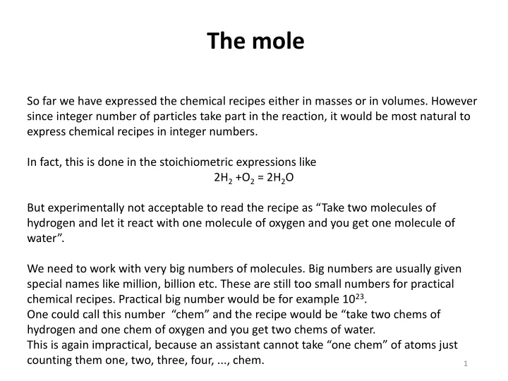
The mole So far we have expressed the chemical recipes either in masses or in volumes. However since integer number of particles take part in the reaction, it would be most natural to express chemical recipes in integer numbers. In fact, this is done in the stoichiometric expressions like 2H2+O2= 2H2O But experimentally not acceptable to read the recipe as Take two molecules of hydrogen and let it react with one molecule of oxygen and you get one molecule of water . We need to work with very big numbers of molecules. Big numbers are usually given special names like million, billion etc. These are still too small numbers for practical chemical recipes. Practical big number would be for example 1023. One could call this number chem and the recipe would be take two chems of hydrogen and one chem of oxygen and you get two chems of water. This is again impractical, because an assistant cannot take one chem of atoms just counting them one, two, three, four, ..., chem. 1
But we know how to make it practical: If we have to buy something like 10000 nails, the shop assistant do not start to count like one, two, three, four,... ,10000. Instead he counts something like 100 nails, then weights (determines the mass) of 100 nails and then gives you nails having 100 times larger mass. And actually if you are experienced carpenter you go to the shop and ask directly for 10 kg of nails, because you have once counted the nails by the above described method. So do the chemists, just they do not use chems but moles . The definition of one mole is: it is the amount of particles which is the same as the amount of molecules in 12 g of carbon isotope 12. So mole is a number, so you have the right to ask how big the number is. It is approximately 6.022x10²³. It took some time to count the number of molecules in one mole, Perrin has got the Nobel price for that, his Nobel lecture is worth to read (http://www.nobelprize.org/nobel_prizes/physics/laureates/1926/perrin- lecture.html). 2
Determining Avogadros number by counting atoms We have said something like an assistant cannot take one chem of atoms just counting them one, two, three, four, ..., chem. It is not quite true. We can determine the Avogadro number by really counting individual atoms. The idea is to count individual radioactive decays using a sample of radioactive element with known half-life. Of course, we cannot take a sample having several grams and counting the clicks of some detectors. We would not distinguish individual decays if the half-life is small or we would have to run the experiment for time exceeding the cosmic age. The idea is to use very small samples with short life times. It is possible to prepare extremely small samples of radioactive liquid easily. The technique is called homeopathic dilution. Take 1 g of radioactive liquid, add 1 g pure water, stir, throw away 1 g of solution. Add 1 g of pure water, stir, throw away 1g. Repeat several times. After N repetitions you would have 1g/2Nradioactive matter in the solution. This can be a very very small number. You could really observe individual decays and count them. If you run the experiment for one halftime, you know the number of radioactive atoms in the solution. If you know the molecular weight you get the Avogadro s number. 3
Ak je rozdiel medzi receptami pre pe enie a chemick mi receptami, pokia ide o nedodr anie presn ch hmotnostn ch pomerov o hovor z kon o st lych zlu ovac ch pomeroch o hovor z kon o mno n ch zlu ovac ch pomeroch Avogadrov z kon o plat o pomeroch hmotnostn ch pomerov v chemick ch receptoch Pre o at mov hmotnosti nie s cel sla o je to m l o je to Avogadrovo slo a ak m ve kos Ak je typick rozmer jednej molekuly Uve te at mov hmotnosti aspo piatich prvkov o to je at mov slo Uve te at mov sla aspo piatich prvkov
Lets repeat, the last two points of the statistical physics manifesto We want to forecast the future at least on the level of macrostates The technique how we handle macrostates in physics is statistics We know the macrostate, but the system is in fact in some unknown microstate There is tremendously huge number of microstates compatible with our information on macrostate A particular macrostate can be realized by tremendously huge number of different microstates. This set of compatible microstates is called a statistical ensemble. We shall see that the number of microstates in an ensemble is of the order 101026. We imagine a procedure which virtually forecast the future of each microstate from the ensemble, make a virtual average and get the average characteristics of the final macrostate which we assume will be the final macrostate of our particular initial macrostate. What justifies usage of the mean value as a reliable prediction? The mean value can be a good strategy if it is very sharp . To observe a microstate with value significantly different from the mean value is in fact highly improbable. So if you want to survive in the jungle , the best advice is to believe to mean values . If you meet something different, well, it s just a bad luck. We shall argue, that such a bad luck is very, very, very improbable. 5
To demonstrate the dominance of the mean value lets consider the following problem from the jungle . I want to open door to entre into the room behind. Well, should I do it? It may happen in principle, that all the molecules of the air inside will, by chance, be all located in the opposite half of the room and I would suffocate. Is that a real danger? Well, no danger at all. The mean value 1:1(division of the molecules between the two halves) is so dominant, that I never find even a tiny difference in pressure between the two halves. We shall demonstrate it using a highly simplified model. Let s assume that each molecule has just two possible states to choose from: be in the left half of the room or in the right half. We shall neglect velocities and the detailed positions of the molecules. Let s calculate the probability ?(?), to find exactly ? molecules left and ? ? molecules right. Note: we have to assume the particles to be distinguishable, since our assumptions are too crude to be used for undistinguishable particles. 6
Obviously: Stirling formula Oh! This looks like a disaster. For large N the probability to find half of the particles in the left half of the room is almost zero! 7
But wait! What we have calculated is the probability for exactly half of the particles in half of the room. This is not something we are interested it in order not to suffocate. What we need is the probability to find something like But even the above inequality describes too many n-s . All those states cannot have the probability roughly equal to the probability of ? =? many of them. There are 0.002 ? 2such states and if each of them had the probability 2, since there is too their summary probability would be Let s be more exact and calculate also the probabilities for ? slightly different from ? 2. 8
denoting n=N/2+x Taylor series in x to the second order gives 9
so for large N we get We have approximated the required sum by an integral, but even the integral cannot be evaluated exactly. What we did is we have approximated the binomial distribution by Gauss distribution. We shall discuss Gauss distributions later it these series of lectures 10
Where erfc() is a special function (complementary error function, consult Wikipedia at http://en.wikipedia.org/wiki/Error_function), which has the following asymptotic behavior for large x for N=1023we get That is the probability to find air pressure by more than 1 per mill higher than it should be. We can really rely on the mean value! Our universe is just exp(40) seconds old! 11
So lets estimate what can be a typical difference between the actual number and the mean number of molecules in the left compartment. The probability is given as So for what values of ? the probability drops significantly as compared to the probability of the mean value ? 2. Clearly it is a value for which the argument in the exponential function will be of the order of -1. This happens for Numerically we get something like So the number of molecules in the left part is constant up to some 12 most significant digits. Really fairly narrow variance with respect to the mean value. Do remember the result: Typical value is of the order ?, typical deviation is of the order ? 12
Lets summarize our findings: mean value of molecules in the left part(as calculated over all the possible microstates) is, as expected ? 2. typical deviation is of the order ? What is the reason for getting this result: Big numbers! The number of molecules is typically ?~1023, a big number The number of possible microstate was 2?~21023a tremendously big number! This situation is typical for statistical physics, we meet there three typical numerical values normal numbers like 1, 4, ??? big numbers like ????, typically number of molecules tremendously big numbers like ??????, typically number of possible microstates 13
Random variables discrete and continuous 14
States, variables, events We shall not discuss here, what we mean by physical system and the state of a physical system Physical variable is roughly any value which characterizes the state of some system, this value can be usually obtained by some measurement. For definiteness one can imagine some measuring apparatus with a digital display. The apparatus is somehow connected to the system and presents a value on its display: this is the value of the variable measured by that apparatus. In classical physics the value of any variable is fully determined by the actual state (microstate) of the system, in quantum physics the value measured by some apparatus is not fully determined by the current state. Obtaining a value of a physical variable needs two things obtaining a state applying the relevant measuring apparatus to the obtained state These two things together we shall call event. 15
Random events Sometimes events (= state + measurement) appear to be (or really are) random. In classical physics everything is in principle deterministic, no space for true randomness there. Still, we are speaking about random events in classical physics as well. What we mean by that? We usually assume that physics experiment should be reproducible, that is starting two experiments in exactly same conditions (same state and same environment) the outcome (event) should be the same. Very often this is not so, the keyword in the preceding sentence is exactly . We simply do not have the initial conditions under the absolute control, so the initial conditions are usually at least slightly different . Sometimes a slight difference in the initial conditions can lead to significant difference in the outcome (event) Then the event looks random, even if there is no true randomness in the game. In quantum mechanics, according to our present state of knowledge, there is true randomness in the measurement process. Measurements on two exactly same states can give different results. Knowing the state exactly, we still cannot deterministically predict the outcome of a measurement, we can only give probabilities for obtaining different values. 16
Random variables If events (= state + measurement) are random, then the values obtained by measurement are also random, we speak about random variables. Be careful and distinguish between event and variable. A variable (even if it is a multidimensional variable) need not characterize the event completely. There might be, for example, two states, giving the same value for the variable considered. So there are two different events having the same value of the variable. So discussing random variables, we have to keep in mind, that the primary notion is random event and random variable is a value (maybe multidimensional) shown in that random event. In what follows we shall distinguish two types of random events discrete continuous In various texts people often do not distinguish between random events and random variable values. Especially for continuous events the event identity (event name) is often given by a value of some (random) variable if the correspondence between the event and the variable value is one-to-one. Even this, however, allows that more then one variable can be associated with the event. 17
From now on in this lecture, we shall consider classical (non-quantum) random events, that is an event is identical to the state. This can be done since the outcome of measurements is fully determined by the state 18
Discrete and continuous random events In any physical experiment, which can lead to random events, we have to identify the set of all possible events which can be the outcome of that experiment. The set of possible events may be finite or countable uncountable (for our purposes with the cardinality of continuum) Using somewhat less precise language we shall use the notions of discrete random events continuous random events To work with probabilities we need unique characterization (naming) of each event. Very often we use as names some numbers, but it is not essential, it is just practical To identify (name) a discrete event, we can use integers. The continuous events cannot be named by integers, we have to use real numbers. To respect some natural structure of the set of continuous events we often use n-tuples off real numbers and we speak about n- dimensional random (continuous) variable. 19
Discrete and continuous random events It is always good to have in mind some specific examples Discrete random event: throwing a dice Continuous random event: throwing a dart If the tip of the dart is absolutely sharp, then it hits just and ideal point of the dartboard, so the event set is continuous. 20
Discrete and continuous random variables According to the definition event = state + measurement; if the event set is discrete then the set of all possible variable values is also discrete, so we speak about discrete random variable if the event set is continuous, the set of variable values might be discrete, but the mathematical treatment we should use is that of continuous random variables in any case Naming the events To identify the events we give them names. Very often we choose some specific variable which uniquely characterizes the event and use the variable value as a name. This variable looks as privileged among other variables, but it is not quite so: the variable just plays two roles. 21
Probability technology: Discrete random variables 22
Discrete random variables Each event in the discrete set can be given a specific name. But since the whole set is countable, the events can also be enumerated or listed, even if the list might be infinite. Enumerability does not mean that we can actually write down the whole infinite list of names, but rather that we can write down a name at any wanted specific position in the list. In principle we can use integers to give names to any countable items, so the list of all the names of an infinite countable sets is just a list of all integers. Probability technology requires, that we can assign a probability to any random event form the list. We shall not define exactly what is the probability, just that any probability is a nonnegative real number and the sum of all the probabilities of events from the list is equal to 1. If we denote the names (imagine integers) of the events as ?, the probabilities as ?(?), we get the conditions 23
The assignment of probabilities can be imagined as a table. For example for our dice example we might get ? ?(?) 1 0.15 2 0.15 3 0.15 4 0.15 5 0.15 6 0.25 We see, that the probabilities are not equal to each other, so the dice is not fair. How we can get (or at least estimate) the probabilities of discrete events? We perform ? experiments and observe how many times ?? the event ? happens. Then 24
Now we shall discuss the variables. So the event ? (with the measurement of the variable ? (number-of-points) gave the value ??. ? ?(?) ?? 1 1 0.15 2 0.15 2 3 0.15 3 4 0.15 4 5 0.15 5 6 0.25 6 By the way, it is easy to imagine a number-of-points-meter. Take a web camera. Make a photo of the dice thrown. Binarize the image to black and white pixels. Count the number of white continuous regions. Show that number on the display as the value for the variable number-of-points. One can easily imagine other variables like square-of-the-number-of-points and even a crazy variable like cosine-of-the-number-of-points. So our table can be extended like this 25
2 ? ?(?) ?? ??= cos?? ??= ?? 1 1 0.15 1 0.540 2 0.15 2 4 -0.416 3 0.15 3 9 -0.990 4 0.15 4 16 -0.654 5 0.15 5 25 0.284 6 0.25 6 36 0.960 In the table like this there one can find the full information about the random system the dice . However, such tables might be huge for some system. Not an easy task to absorb the information in one s had. So very often, we chose to present reduced information, even squeezed to just one number: the mean value. The mean value of the random variable ? is defined as 26
Notice, that using the experimental determination of probability we get and this is exactly how we all used to calculate the average mark in the school: if you got 3 one s and 4 two s you calculated Also be aware that the formula for the mean value is not a natural law . Nature is not aware of any such rule. The formula is our human definition. Well, it is not a completely arbitrary definition. We had some good reasons why we defined it like that, but we could chose something else equally well. For example sometimes we use the median value for very similar purpose as we use the mean value . 27
In statistics and probability theory, the median is the numerical value separating the higher half of a probability distribution (a data sample, a population), from the lower half. Denoting the median value of the variable ? as ?, we define it by the following: define the set of indices (names of random events) denoted by Low(?) as the set of all ? for which ?? ? define the set of indices (names of random events) denoted by Hi(?) as the set of all ? for which ?? ? Define median ? as any number for which and simultaneously Do think over this definition and you find that it corresponds to the above mentioned informal definition . Just you have to accept, that in some situations the median value is not defined uniquely (that is why the words any number and not the number in the formal definition). There are situations where the median value is more descriptive then the mean value. 28
Reducing the information about some probabilistic distribution to just one number, the mean value (or the median value) is very often too crude a reduction. We would like to know at least how different the individual random values are from the mean value. Something like a typical difference between a specific random value and the mean value. For this purpose we define a standard deviation as the square root of variance. The variance ?2itself is defined as a mean square of deviation (or mean deviation squared). So the standard deviation is defined as 29


 is a special function (complementary error")