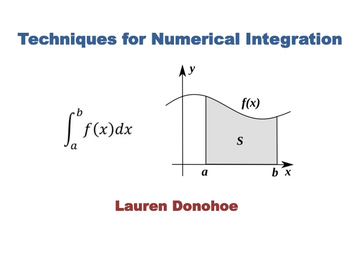
Techniques for Numerical Integration by Lauren Donohoe
Learn about various numerical integration techniques such as Trapezoid Rule, Simpson's Rule, Romberg Integration, and Gaussian Quadrature. Understand the basics of integrals, interpolation polynomials, and the application of these techniques for accurate calculations.

Download Presentation

Please find below an Image/Link to download the presentation.
The content on the website is provided AS IS for your information and personal use only. It may not be sold, licensed, or shared on other websites without obtaining consent from the author.If you encounter any issues during the download, it is possible that the publisher has removed the file from their server.
You are allowed to download the files provided on this website for personal or commercial use, subject to the condition that they are used lawfully. All files are the property of their respective owners.
The content on the website is provided AS IS for your information and personal use only. It may not be sold, licensed, or shared on other websites without obtaining consent from the author.
E N D
Presentation Transcript
Techniques for Numerical Integration Techniques for Numerical Integration Lauren Donohoe Lauren Donohoe
Numerical Integration Techniques Trapezoid Rule Simpson s Rule(s) Romberg Integration Gaussian Quadrature Gauss-Lobatto Quadrature Gauss-Kronrod Quadrature MATLAB Comparison trapz() simps() quad() romberg() quadl() quadgk() integral() Working with Singularities
The Integral The Basics What you already know Indefinite Integral: Definite Integral: On the closed interval from a to b, or [a,b] Integral - Area Under the Curve The Fundamental Theorem of Calculus: If f(x) is a continuous, real-valued function defined on the closed interval [a,b], and F(x) is defined for all x in [a,b], then F(x) is differentiable on (a,b)
The Interpolation Polynomial The simple approach to Numerical Integration Let pn(x) be the polynomial to interpolate f(x) at x0,x1, ,xn where Then use this interpolation polynomial to compute f(x) by using Where a = x0 and b = xn. Then taking the form the function In(f) takes the exact value of the integral for polynomials of degree n or less Represented as a linear system
The Interpolation Polynomial - Applied The first example If we let [a,b] = [0,1], xk = kh where h = 1/n For n = 1 then X0 = 0 and x1 = 1, Has solution C0 = C1 = , and plugging this back into the equation for the polynomial, Or more generally:
The Trapezoid Rule A technique for approximating the definite integral The trapezoid rule approximates the area under the curve as a trapezoid with upper corners on the curve, and determines the value for the interval using the area of the trapezoid formed. (only ONE trapezoid, for now) Q = trapz(Y) returns the approximate integral of Y using the trapezoid method (by default, with unit spacing)
The Interpolation Polynomial - Applied The second example If we continue to let [a,b] = [0,1], xk = kh where h = 1/n For n = 2 then X0 = 0, x1 = and x2 = 1, Has solution C0 = C2 = 1/6, and C1 = 2/3 and plugging this into the polynomial, Or more generally:
Simpsons Rule A better technique for approximating the definite integral Simpson s rule approximates the area under the curve using quadratic interpolation [ Parabolic arcs rather than straight lines ] Simpson 3/8 Rule (n = 3) Simpson s 3/8 rule approximates the area under the curve using cubic interpolation rather than quadratic interpolation
Newton-Cotes & Error Formulas Recap: Interpolation Formula is used to approximate integrals in numerical analysis n = 1 Trapeziod rule n = 2 Simpson s rule n = 3 Simpson s 3/8 Rule x0, x1, , xn are evenly spaced For unevenly spaced points, Gaussian Quadrature is necessary. n = 4, 5, 6, Newton Cotes Formula of order n (Guaranteed exact for degree n or less) Error Formulas: Trapezoid Rule Simpson s Rule
Composite Formulas A MUCH better technique for approximating the definite integral As n increases, the different Newton-Coates formulas help us to approximate the value of the integral of more complex curves, represented by higher order polynomials. Composite = Break the integral up into smaller integrals and sum the parts In general, the more parts , the better the approximation.
Composite Trapezoid Rule For notation simplicity using spacing h = xk+1 xk = (b-a) Therefore, to halve the interval size, midpoints:L xk+1/2 = [xk + xk+1]/2 Q = trapz(X,Y) returns the approximate integral of Y using the trapezoid method with spacing X
Adaptive Simpsons Rule Composite = Break the integral up into smaller integrals and sum the parts Adaptive = Recursively splitting the integral in half and checking the error term compared to some desired maximum value Q = quad(fun,a,b,tol) returns the approximate integral of the function fun using recursive adaptive composite Simpson s Rule to within an error of tol (larger tolerance values means fewer evaluations and faster computation but a less accurate result
Romberg Integration Combining everything up until this point The composite trapezoid rule for spacing h was And with half the interval size, need the function evaluated at the midpoints To(h) is needed in order to determine To(h/2) It follows that in order to compute To(h/2k) we need To(h). To(h/2), , To(h/2k) Following the same process to determine the composite Simpson s rule has the result Similarly, To(h/4 ) and To(h/2) are needed to form T1(h/2), and so forth Then again in the same way, T1(h) and T1(h/2) can be used to determine T2(h) [ This technique of using multiple low order approximations to obtain a higher order approximation is called Richardson Extrapolation. ]
Romberg Integration Richardson Extrapolation + Trapezoid Rule = Romberg Integration Such that finally, the general form Which can be used with the table in order to form the flow of the algorithm. The rows The columns The diagonals ALL converge to the exact value of the integral Stopping Criterion for some tolerance
Gaussian Quadrature A slightly different technique for approximating the definite integral Quadrature is a numerical analysis technique where a definite integral is approximated using a weighted sum of function values at specified points within the domain of integration The n-point Gaussian Quadrature rule yields exact results for polynomials of degree (2n-1) or less as long as a suitable choice of points xi and weights wi are used for i = 1,2, ,n The domain is conventionally used as the closed interval [-1,1] How is this different? These specified points DO NOT have to be evenly spaced (as they did for Trapezoid, Simpson s, and Romberg)
Gaussian Quadrature using a suitable choice of points xi and weights wi Gaussian Quadrature will produce accurate results if the function f(x) is well approximated by a polynomial function within the domain [This method is not well suited for functions with singularities ] If f(x) can be written as f(x) = w(x)g(x) where g(x) can be well approximated using a polynomial and w(x) is known, then alternative points and weights that depend on the weighing function give better results and the evaluation points xi are the roots (zeros) the specific polynomial used to approximate the function, a polynomial belonging to a family of orthogonal polynomials called the orthogonal polynomial sequence
Gaussian Quadrature Weighing Functions Quadrature Type Weighing Function w(x) Orthogonal Polynomials Gauss-Legendre Quadrature 1 Legendre Polynomials Gauss-Jacobi Quadrature Jacobi Polynomials Chebyshev-Gauss Quadrature Chebyshev Polynomials (first kind) Chebyshev-Gauss Quadrature Chebyshev Polynomials (second kind) Gauss-Laguerre Quadrature Laguerre Polynomials Gauss-Laguerre Quadrature Generalized Laguerre Polynomials Gauss-Hermite Quadrature Hermite Polynomials
Gauss Lobatto Quadrature An Extension of Gaussian Quadrate How is Gauss-Lobatto different than Gaussian Quadrature? - The integration points INCLUDE the endpoints of the integration interval - Accurate for polynomials up to degree 2n-3 The Lobatto Quadrature of the function f(x) on the interval [-1,1] is with weights and remainder q = quadl(fun,a,b) approximates the integral of the function fun from a to b, to within an error of 10-6using adaptive Lobatto quadrature. (Limits a and b must be finite.)
Gauss Kronrod Quadrature Another Extension of Gaussian Quadrate Remember: Gaussian Quadrature of order n is accurate for polynomials up to degree 2n-1 Gauss-Kronrod Rules: Adding n+1 points to an n-point Quadrature, in this manner makes the resulting rule of order 3n+1. This allows for computation of much higher-order estimates using function values of lower-order estimates The interval [a,b] is subdivided such that the new evaluation points of these subintervals never coincide with the original evaluation points except at zero and odd numbers q = quadgk(fun,a,b) approximates the integral of the function fun from a to b using high-order adaptive quadrature with default error tolerances. (Limits a and b can be infinite or complex.)
MATLAB Comparison - Results Time Elapsed (seconds) MATLAB Function Integral Value Error Trapezoid Rule 3 0.14159 0.02266 trapz() Simpson s Rule 3.1333 0.0082593 0.030717 simps() * Adaptive Composite Simpson Quadrature 3.14159525048309 2.5969e-06 0.023679 quad() Romberg Integration (with tolerance 0.1) 3.141592502458707 1.5113e-07 0.001437 romberg() * Romberg Integration (with tolerance 1e-14) 3.141592653589793 0 0.014495 romberg() * Gauss-Lobatto Quadrature 3.141592707032192 5.3442e-08 0.02867 quadl() Gauss-Kronrod Quadrature 3.141592653589793 0 0.067964 quadgk() MATLAB s Integral Function 3.141592653589793 0 0.089876 integral() = 3.1415926535897932384626 Zero to double precision
Differences in MATLAB Functions Which function should I use to perform numerical integration? - quad() is more efficient for low accuracy with non-smooth scalar-valued functions - quadl() is more efficient for higher accuracy with smooth scalar-valued functions - quadv() & integral() perform vectorized quadrature for a vector-valued function - quadgk() is the most efficient for high accuracy if the function is oscillatory - quadgk() & integral() supports infinite limits of integration - quadgk() & integral() can handle moderate singularities at the endpoints - integral() automatically supports mixed relative (digits) and absolute (when I = 0) error control - integral() uses a higher order method than quadl() so it is usually more accurate on smooth problems - integral() is more reliable than quad() because it starts with a much finer initial mesh than quad() and is more conservative in error control
Handling Singularities in MATLAB - quadgk() & integral() can handle moderate singularities at the endpoints - quad() is more efficient for low accuracy with non-smooth scalar-valued functions If there is a singularity within the domain of the function, the sum of the intervals over multiple subintervals can be used with the singularities at endpoints The Dirac-Delta Function Without Split With Split quad() a = 1e-20 * a = 1e-21 quadgk() a = 1e-4 a = 1e-7 integral() a = 1e-4 a = 1e-7 *
Pocklingtons Integral Equation Using MATLAB to evaluate Pocklington s Integral Equation Using piecewise triangular sub-domain functions = otherwise ; 0 | ;| z z + n z z z ( ) z n n f n And point-matching (or collocation) weighing functions ) ( m z w = ( ) z z m The kernel of Pocklington s I.E. has a singularity at the middle segment of the dipole 0 4 R j jkR 1 e = + + 2 2 2 2 2 ( , ) 1 ( )( 2 3 ) K z z jkR R a k a R m 5 2) = + 2 ( R z z a
Pocklingtons I.E. FEKO Singularity on the center segment Splitting the integral does not help Comparison of impedances (center segment) MATLAB
References http://www.mathstat.dal.ca/~tkolokol/classes/1500/romberg.pdf http://en.wikipedia.org/wiki/Integral#Fundamental_theorem_of_calculus_2 http://en.wikipedia.org/wiki/Polynomial_interpolation http://en.wikipedia.org/wiki/Simpson%27s_rule http://en.wikipedia.org/wiki/Newton%E2%80%93Cotes_formulas http://www.cse.psu.edu/~barlow/cse451/classnotes.html Advanced Mathematics and Mechanics Applications Using MATLAB, Third Edition By David Halpern, Howard B. Wilson, Louis H. Turcotte Advanced Engineering Mathematics with MATLAB, Third Edition By Dean G. Duffy http://en.wikipedia.org/wiki/Trapezoidal_rule http://www.mathworks.com/matlabcentral/fileexchange/25754-simpsons-rule-for-numerical- integration/content/simps.m http://www.mathworks.com/help/matlab/ http://ezekiel.vancouver.wsu.edu/~cs330/lectures/integration/simpsons.pdf