Regression Analysis in Predictive Modeling

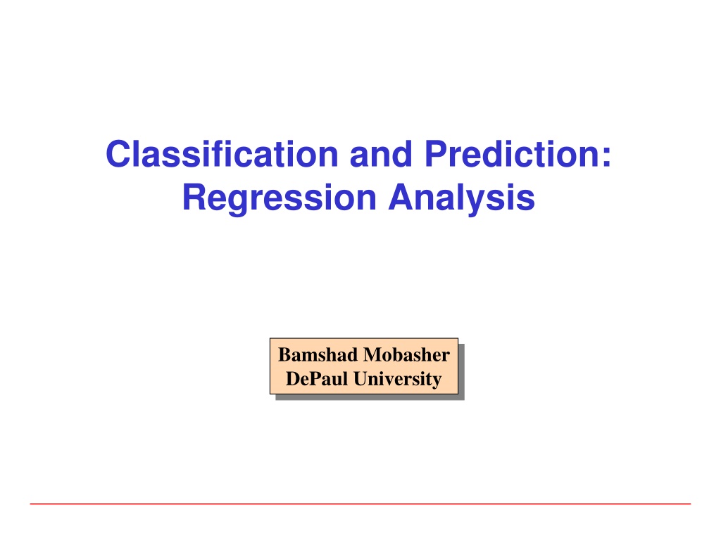
Classification and Prediction: Regression Analysis Bamshad Mobasher DePaul University

What Is Numerical Prediction (a.k.a. Estimation, Forecasting) (Numerical) prediction is similar to classification construct a model use model to predict continuous or ordered value for a given input Prediction is different from classification Classification refers to predicting categorical class label Prediction models continuous-valued functions Major method for prediction: regression model the relationship between one or more independent or predictor variables and a dependent or response variable Regression analysis Linear and multiple regression Non-linear regression Other regression methods: generalized linear model, Poisson regression, log-linear models, regression trees 2

Linear Regression Linear regression: involves a response variable y and a single predictor variable x y = w0 + w1 x y x Goal: Using the data estimate weights (parameters) w0 and w1 for the line such that the prediction error is minimized The weights w0 (y-intercept) and w1 (slope) are regression coefficients 3

Linear Regression w y = 0+ w x 1 y Observed Value of y for xi ei Slope = w1 Predicted Value of y for xi Error for this x value Intercept = w0 x xi

Linear Regression Method of least squares: Estimates the best-fitting straight line w0 and w1 are obtained by minimizing the sum of the squared errors (a.k.a. residuals) 2 = = 2 y ( ) SSE e y i i i i i = + 2 ( ( )) y w w x 0 1 i i w1 can be obtained by setting the partial derivative of the SSE to 0 and solving for w1, ultimately resulting in: i ( )( ) x x y y = i i w = w y w x i 0 1 1 2 ( ) x x i 5

Multiple Linear Regression Multiple linear regression: involves more than one predictor variable Features represented as x1, x2, , xd Training data is of the form (x1, y1), (x2, y2), , (xn, yn) (each xj is a row vector in matrix X, i.e. a row in the data) For a specific value of a feature xi in data item xj we use: Ex. For 2-D data, the regression function is: j ix = + + y w w x w x 0 1 1 2 2 y x2 x1 6

Least Squares Generalization Multiple dimensions To simplify add a new feature x0 = 1 to feature vector x: x1 x0 x2 y 1 1 1 1 1 d d = i = i = = + = = T w . x y ( , ,..., ) f x x x w x w x w x 0 1 0 0 d i i i i 1 0

Least Squares Generalization d d = i = i = = = + = = T x w x . y ( , ,..., ) ( ) f x x x f w x w x w x 0 1 0 0 d i i i i 1 0 Calculate the error function (SSE) and determine w: 2 d n d ( ) = i = j = i 2 = = = 2 i j w y x y ( ) ( ) ( ) E f w x y w x i i i i 0 1 0 = T y Xw y Xw ( ) ( = ) j y vector of training all responses y = j X x = matrix of training all samples T 1 T w X = X X y for test ( ) Closed form solution to w wE test test test w x x y sample = ( ) 0

Extending Application of Linear Regression The inputs X for linear regression can be: Original quantitative inputs Transformation of quantitative inputs, e.g. log, exp, square root, square, etc. Polynomial transformation example: y = w0 + w1 x + w2 x2 + w3 x3 Dummy coding of categorical inputs Interactions between variables example: x3 = x1 x2 This allows use of linear regression techniques to fit much more complicated non-linear datasets.

Example of fitting polynomial curve with linear model

Regularization Complex models (lots of parameters) are often prone to overfitting Overfitting can be reduced by imposing a constraint on the overall magnitude of the parameters (i.e., by including coefficients as part of the optimization process) Two common types of regularization in linear regression: L2 regularization (a.k.a. ridge regression). Find w which minimizes: = = j i 1 0 N d d = i 2 + 2 ( ) y w x w j i i i 1 is the regularization parameter: bigger imposes more constraint L1 regularization (a.k.a. lasso). Find w which minimizes: = = j i 1 0 N d d = i + 2 ( ) | | y w x w j i i i 1

Other Regression-Based Models Generalized linear models Foundation on which linear regression can be applied to modeling categorical response variables Variance of y is a function of the mean value of y, not a constant Logistic regression: models the probability of some event occurring as a linear function of a set of predictor variables Poisson regression: models the data that exhibit a Poisson distribution Log-linear models (for categorical data) Approximate discrete multidimensional prob. distributions Also useful for data compression and smoothing Regression trees and model trees Trees to predict continuous values rather than class labels 12

Regression Trees and Model Trees Regression tree: proposed in CART system (Breiman et al. 1984) CART: Classification And Regression Trees Each leaf stores a continuous-valued prediction It is the average value of the predicted attribute for the training instances that reach the leaf Model tree: proposed by Quinlan (1992) Each leaf holds a regression model a multivariate linear equation for the predicted attribute A more general case than regression tree Regression and model trees tend to be more accurate than linear regression when instances are not represented well by simple linear models 13

Evaluating Numeric Prediction Prediction Accuracy Difference between predicted scores and the actual results (from evaluation set) Typically the accuracy of the model is measured in terms of variance (i.e., average of the squared differences) Common Metrics (pi = predicted target value for test instance i, ai = actual target value for instance i) Mean Absolute Error: Average loss over the test set + + ( ) ... ( ) p a p a = 1 1 n n MAE n Root Mean Squared Error: compute the standard deviation (i.e., square root of the co-variance between predicted and actual ratings) + + 2 2 ( ) ... ( ) p a p a = 1 1 n n RMSE n 14

Example: Web Traffic Data 15

1D Poly Fit Example of too much bias underfitting 16

Example: 1D and 2D Poly Fit 17

Example: 1D Ploy Fit Example of too much variance overfitting 18

Bias-Variance Tradeoff 19

Bias-Variance Tradeoff Possible ways of dealing with high bias Get additional features More complex model (e.g., adding polynomial terms such as x12, x22 , x1.x2, etc.) Use smaller regularization coefficient . Note: getting more training data won t necessarily help in this case Possible ways dealing with high variance Use more training instances Reduce the number of features Use simpler models Use a larger regularization coefficient . 20