Ray Tracing Techniques in Computer Graphics
 undefined


Ray Tracing
CMSC 635


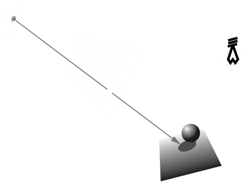
Basic idea
How many intersections?
Pixels
~10
3
to ~10
7
Rays per Pixel
1 to ~10
Primitives
~10 to ~10
7
Every ray vs. every primitive
~10
4
to ~10
15
Speedups
Fewer intersections
Faster intersections
Fewer Intersections:
Algorithmic improvements
Object-based
Decide ray doesn’t intersect early
Still intersect along full ray length
Space-based
Partial order of intersection tests
Terminate ray early
Image-based
Ray-to-ray coherence
Object: bounding hierarchy
Bounding spheres
AABB
OBB
K-DOP
Bounding spheres
Very fast to intersect
Hard to fit
Poor fit
AABB
Fast to intersect
Easy to fit
Reasonable fit
OBB
Pretty fast to
intersect
Harder to fit
Eigenvectors of
covariance matrix
Iterative minimization
Good fit
K-DOP
K-Dimensional
Oriented Polytope
All objects use same
K parallel planes
Creation & test cost
between AABB and
OBB
Space: partitioning
Uniform grid
BSP
Octtree
K-D tree
Uniform Grid
Fast to traverse
Steps in X, Y & Z
Scale problems
“teapot in a stadium”
Same object in
multiple cells
Mailboxing
BSP : Binary Space Partition
Binary Tree
Arbitrary Planar
Splits
Body
Octree
Axis-aligned cells
8-children per node
2D: Quadtree
K-D Tree
Axis-aligned splits
Arbitrary locations
Image
Coherence
Light buffer (avoid shadow rays)
Pencil tracing/cone tracing
Image approximation
Truncate ray tree
Successive refinement
Contrast-driven antialiasing
Faster intersections
Store partial precomputation with object
Stop early for reject
Postpone expensive operations
Reject then normalize
If a cheap approximate test exists, do it first
Sphere / box / separating axes / …
Project to fewer dimensions
Cache results from previous tests
Mailboxing
Intersection approaches
Plug parametric ray into implicit shape
Plug parametric shape into implicit ray
Solve implicit ray = implicit shape
Making it easier
Transform to cannonical ray
(0,0,0)–(0,0,1)
Transform to cannonical object
Ellipsoid to unit sphere at (0,0,0)
Compute in stages
Polygon plane, then polygon edges
Numerical iteration
Parallel intersections
Distribute pixels
Distribute rays
Distribute objects
Distribute space
Parallel intersections
Load balancing
Scattered rays, blocks, lines, ray queues
Culling
Communication costs
Database
Ray requests
Ray results
Assigned papers
Cook et al. 1984
Amanatides and Woo 1987
Wald et al. 2006 (or 2007?)
Popov et al. 2009
Pantaleoni and Luebke 2010
Cook et al. 1984
Distributed Ray Tracing
Explosion of samples
Antialiasing, Glossy reflections,
Translucency, Soft shadows, Depth of
field, Motion blur
Ray makes a random choice for each
Version of Monte Carlo integration
Cook et al. 1984
Cook et al. 1984
Cook et al. 1984
Amanatides and Woo 1987
Steps along each axis are uniform
Just need to pick which one
Don’t repeat intersection computations
Ray IDs, store with object
Wald et al. 2007
Trace a collection of rays through a grid
Use frustum of ray packet
Trace one slice at a time
Popov et al. 2009
Compare AABB to K-D tree
Surface Area Heuristic
Nest, share or split between nodes?
Grid for speed
Axis aligned sweeps
Pantaleoni and Luebke 2010
Morton code (also called Z order)
Naturally nests
Talks about surface area heuristic
Dynamic geometry
Full resort every frame
Explore the fundamentals of ray tracing, including concepts like intersections, speedups, fewer intersections strategies, object bounding hierarchies, and space partitioning methods for efficient rendering. Learn about bounding spheres, AABBs, OBBs, K-DOPs, uniform grids, BSP trees, and octrees in the context of optimizing ray tracing algorithms.

Download Presentation

Please find below an Image/Link to download the presentation.
The content on the website is provided AS IS for your information and personal use only. It may not be sold, licensed, or shared on other websites without obtaining consent from the author.If you encounter any issues during the download, it is possible that the publisher has removed the file from their server.
You are allowed to download the files provided on this website for personal or commercial use, subject to the condition that they are used lawfully. All files are the property of their respective owners.
The content on the website is provided AS IS for your information and personal use only. It may not be sold, licensed, or shared on other websites without obtaining consent from the author.
E N D
Presentation Transcript
CMSC 635 Ray Tracing
How many intersections? Pixels ~103to ~107 Rays per Pixel 1 to ~10 Primitives ~10 to ~107 Every ray vs. every primitive ~104to ~1015
Speedups Fewer intersections Faster intersections
Fewer Intersections: Algorithmic improvements Object-based Decide ray doesn t intersect early Still intersect along full ray length Space-based Partial order of intersection tests Terminate ray early Image-based Ray-to-ray coherence
Object: bounding hierarchy Bounding spheres AABB OBB K-DOP
Bounding spheres Very fast to intersect Hard to fit Poor fit
AABB Fast to intersect Easy to fit Reasonable fit
OBB Pretty fast to intersect Harder to fit Eigenvectors of covariance matrix Iterative minimization Good fit
K-DOP K-Dimensional Oriented Polytope All objects use same K parallel planes Creation & test cost between AABB and OBB
Space: partitioning Uniform grid BSP Octtree K-D tree
Uniform Grid Fast to traverse Steps in X, Y & Z Scale problems teapot in a stadium Same object in multiple cells Mailboxing
BSP : Binary Space Partition Binary Tree Arbitrary Planar Splits Body Arm Head Arm Leg Leg
Octree Axis-aligned cells 8-children per node 2D: Quadtree
K-D Tree Axis-aligned splits Arbitrary locations
Image Coherence Light buffer (avoid shadow rays) Pencil tracing/cone tracing Image approximation Truncate ray tree Successive refinement Contrast-driven antialiasing
Faster intersections Store partial precomputation with object Stop early for reject Postpone expensive operations Reject then normalize If a cheap approximate test exists, do it first Sphere / box / separating axes / Project to fewer dimensions Cache results from previous tests Mailboxing
Intersection approaches Plug parametric ray into implicit shape Plug parametric shape into implicit ray Solve implicit ray = implicit shape
Making it easier Transform to cannonical ray (0,0,0) (0,0,1) Transform to cannonical object Ellipsoid to unit sphere at (0,0,0) Compute in stages Polygon plane, then polygon edges Numerical iteration
Parallel intersections Distribute pixels Distribute rays Distribute objects Distribute space
Parallel intersections Load balancing Scattered rays, blocks, lines, ray queues Culling Communication costs Database Ray requests Ray results
Assigned papers Cook et al. 1984 Amanatides and Woo 1987 Wald et al. 2006 (or 2007?) Popov et al. 2009 Pantaleoni and Luebke 2010
Cook et al. 1984 Distributed Ray Tracing Explosion of samples Antialiasing, Glossy reflections, Translucency, Soft shadows, Depth of field, Motion blur Ray makes a random choice for each Version of Monte Carlo integration
Amanatides and Woo 1987 Steps along each axis are uniform Just need to pick which one Don t repeat intersection computations Ray IDs, store with object
Wald et al. 2007 Trace a collection of rays through a grid Use frustum of ray packet Trace one slice at a time
Popov et al. 2009 Compare AABB to K-D tree Surface Area Heuristic Nest, share or split between nodes? Grid for speed Axis aligned sweeps
Pantaleoni and Luebke 2010 Morton code (also called Z order) Naturally nests Talks about surface area heuristic Dynamic geometry Full resort every frame