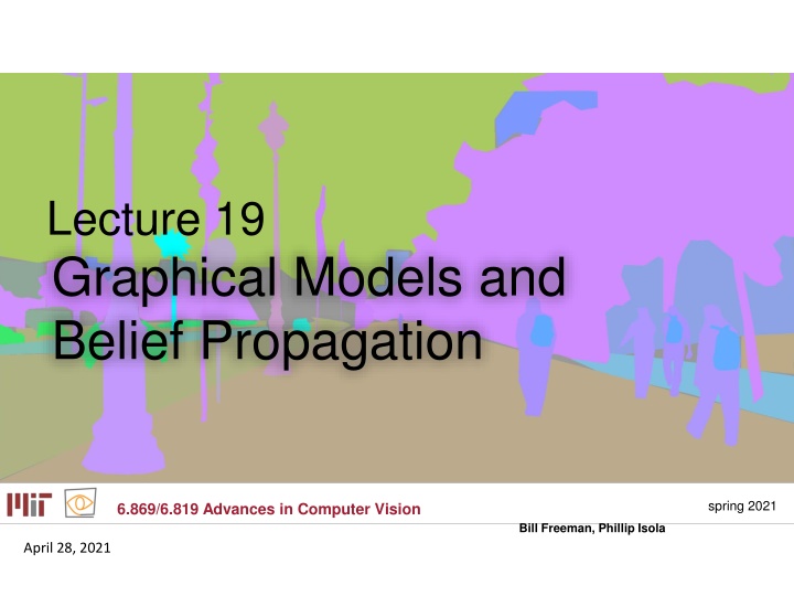
Graphical Models and Belief Propagation in Computer Vision

Lecture 19

Graphical Models and

Belief Propagation

April 28, 2021

Identical local evidence...

…different interpretations

Local

information...

...must propagate

Probabilistic graphical models are a powerful tool for propagating

information within an image.  And these tools are used everywhere

within computer vision now.

Information must propagate over

the image.

From a random sample of 6

papers from CVPR 2014, half

had figures that look like this...

7

http://www.cvpapers.com/cvpr2014.html

8

http://hci.iwr.uni-heidelberg.de/Staff/bsavchyn/papers/swoboda-

GraphicalModelsPersistency-with-Supplement-cvpr2014.pdf

Partial Optimality by Pruning for MAP-inference with General

Graphical Models, Swoboda et al

9

file:///Users/billf/Downloads/dewarp_high.pdf

Active flattening of curved document images via two

structured beams, Meng et al.

A Mixture of Manhattan Frames: Beyond the Manhattan

World, Straub et al

10

http://www.jstraub.de/download/straub2014mmf.pdf

Undirected graphical models

•

A set of nodes joined by undirected edges.

•

The graph makes conditional independencies explicit:  If two

nodes are not linked, and we condition on every other node in the

graph, then those two nodes are conditionally independent.

Conditionally independent, because

are not connected by a line in the

undirected graphical model

11

Undirected graphical models:  cliques

•

Clique:  a fully connected set of nodes

•

A maximal clique is a clique that can’t include more nodes of the

graph w/o losing the clique property.

M

a

x

i

m

a

l

c

l

i

q

u

e

n

o

t

a

c

l

i

q

u

e

N

o

n

-

m

a

x

i

m

a

l

c

l

i

q

u

e

c

l

i

q

u

e

12

Undirected graphical models:

probability factorization

•

Hammersley-Clifford theorem addresses the pdf factorization

implied by a graph:  A distribution has the Markov structure

implied by an undirected graph iff it can be represented in the

factored form

s

e

t

o

f

m

a

x

i

m

a

l

c

l

i

q

u

e

s

P

o

t

e

n

t

i

a

l

f

u

n

c

t

i

o

n

s

o

f

s

t

a

t

e

s

o

f

v

a

r

i

a

b

l

e

s

i

n

m

a

x

i

m

a

l

c

l

i

q

u

e

N

o

r

m

a

l

i

z

i

n

g

c

o

n

s

t

a

n

t

13

e

d

g

e

s

c

o

n

n

e

c

t

i

n

g

n

o

d

e

s

s

e

t

o

f

n

o

d

e

s

Graphical Models

M

a

r

k

o

v

R

a

n

d

o

m

F

i

e

l

d

s

14

Markov Random Fields (MRF)

•

Oftentimes MRF’s have a regular, grid-like

structure (but they don’t need to).

15

MRF nodes as pixels

Winkler, 1995, p. 32

16

MRF nodes as patches

image patches



(

x

i

, y

i

)



(

x

i

, x

j

)

image

scene

scene patches

17

Network joint probability

scene

image

Scene-scene

compatibility

function

neighboring

scene nodes

local 

observations

Image-scene

compatibility

function











i

i

i

j

i

j

i

y

x

x

x

Z

y

x

P

)

,

(

)

,

(

1

)

,

(

,

18

Energy formulation

19

scene

image

Scene-scene

compatibility

function

neighboring

scene nodes

local 

observations

Image-scene

compatibility

function

22

In order to use MRFs:

20

23

Markov Random Fields (MRF’s)

•

Inference in MRF’s.

–

Gibbs sampling, simulated annealing

–

Iterated conditional modes (ICM)

–

Belief propagation

•

Application example—super-resolution

–

Graph cuts

–

Variational methods

•

Learning MRF parameters.

–

Iterative proportional fitting (IPF)

21

24

Outline of MRF section

•

Inference in MRF’s.

–

Gibbs sampling, simulated annealing

–

Iterated conditional modes (ICM)

–

Belief propagation

•

Application example—super-resolution

–

Graph cuts

–

Variational methods

•

Learning MRF parameters.

–

Iterative proportional fitting (IPF)

22

•

Gibbs sampling:

–

A way to generate random samples from a (potentially

very complicated) probability distribution.

–

Fix all dimensions except one.  Draw from the resulting

1-d conditional distribution.  Repeat for all dimensions,

and repeat many times.

–

Take an average of a subset of those samples to

estimate the posterior mean.  (Wait for a “burn in”

period before including samples.  And then subsample

Gibbs sampler outputs to find independent draws of the

joint probability).

Gibbs Sampling

Reference:  Geman and Geman, IEEE PAMI 1984.

23

26

Sampling from a 1-d function

24

Gibbs Sampling

Slide by Ce Liu

25

•

Gibbs sampling:

–

A way to generate random samples from a (potentially

very complicated) probability distribution.

–

Fix all dimensions except one.  Draw from the resulting

1-d conditional distribution.  Repeat for all dimensions,

and repeat many times

•

Simulated annealing:

–

A schedule for modifying the probability distribution so

that, at “zero temperature”, you draw samples only

from the MAP solution.

Gibbs Sampling and Simulated Annealing

Reference:  Geman and Geman, IEEE PAMI 1984.

26

Gibbs sampling and simulated

annealing

27

Gibbs sampling and simulated

annealing

28

•

Inference in MRF’s.

–

Gibbs sampling, simulated annealing

–

Iterated conditional modes (ICM)

–

Belief propagation

•

Application example—super-resolution

–

Graph cuts

•

Application example--stereo

–

Variational methods

•

Application example—blind deconvolution

•

Learning MRF parameters.

–

Iterative proportional fitting (IPF)

Outline of MRF section

29

Iterated conditional modes

Described in:  Winkler, 1995.  Introduced by Besag in 1986.

30

Winkler, 1995

31

•

Inference in MRF’s.

–

Gibbs sampling, simulated annealing

–

Iterated conditional modes (ICM)

–

Loopy belief propagation

•

Application example—super-resolution

–

Graph cuts

–

Variational methods

•

Learning MRF parameters.

–

Iterative proportional fitting (IPF)

Outline of MRF section

32

Derivation of belief propagation

33

The posterior factorizes

34

Propagation rules

35

Propagation rules

36

Propagation rules

37

Belief propagation messages

j

i

i

=

j

To send a message

:  Multiply together all the incoming

messages, except from the node you’re sending to,

then multiply by the compatibility matrix and marginalize

over the sender’s states.

A message

:  can be thought of as a set of weights on

each of your possible states

38

Beliefs

j

To find a node’s beliefs

:  Multiply together all the

messages coming in to that node.

39

Max-product belief propagation

40

•

“Do the right thing” Bayesian algorithm.

•

For Gaussian random variables over time:

Kalman filter.

•

For hidden Markov models:

forward/backward algorithm (and MAP

variant is Viterbi).

Optimal solution in a chain or tree:

Belief Propagation

41

Belief, and message update rules are just

local operations, and can be run whether

or not the network has loops

j

i

i

=

j

42

Justification for running belief propagation in networks with loops

•

Experimental results:

–

Comparison of methods

–

Error-correcting codes

–

Vision applications

•

Theoretical results:

–

For Gaussian processes, means are correct.

–

Large neighborhood local maximum for MAP.

–

Equivalent to Bethe approx. in statistical physics.

–

Tree-weighted reparameterization

Weiss and Freeman, 2000

Yedidia, Freeman, and Weiss, 2000

Freeman and Pasztor, 1999;

Frey, 2000

Kschischang and Frey, 1998;

McEliece et al., 1998

Weiss and Freeman, 1999

Wainwright, Willsky, Jaakkola, 2001

Szeliski et al. 2008

43

http://vision.middlebury.edu/MRF/

testMRF.m

Show program comparing some

methods on a simple MRF

44

•

Inference in MRF’s.

–

Gibbs sampling, simulated annealing

–

Iterated conditional modes (ICM)

–

Belief propagation

•

Application example—super-resolution

–

Graph cuts

–

Variational methods

•

Learning MRF parameters.

–

Iterative proportional fitting (IPF)

Outline of MRF section

45

53

Super-resolution

•

Image:  low resolution image

•

Scene:  high resolution image

ultimate goal...

46

Polygon-based

graphics

images are

resolution

independent

47

3 approaches to perceptual

sharpening

(1)  Sharpening;  boost existing high

frequencies.

(2)  Use multiple frames to obtain

higher sampling rate in a still frame.

(3)  Estimate high frequencies not

present in image, although implicitly

defined.

In this talk, we focus on (3), which

we’ll call “super-resolution”.

spatial frequency

amplitude

spatial frequency

amplitude

48

•

 Schultz and Stevenson, 1994

•

 Pentland and Horowitz, 1993

•

fractal image compression (Polvere, 1998; Iterated Systems)

•

astronomical image processing (eg. Gull and Daniell, 1978;

“pixons” 

http://casswww.ucsd.edu/puetter.html

)

•

Follow-on:  Jianchao Yang, John Wright, Thomas S. Huang,

Yi Ma: Image super-resolution as sparse representation of raw

image patches. CVPR 2008

Super-resolution: other approaches

49

57

Training images,

~100,000 image/scene patch pairs

Images from two Corel database categories:

“giraffes” and “urban skyline”.

50

Do a first interpolation

Zoomed low-resolution

Low-resolution

51

Zoomed low-resolution

Low-resolution

Full frequency original

52

Full freq. original

Representation

Zoomed low-freq.

53

61

True high freqs

Low-band input

(contrast normalized,

PCA fitted)

Full freq. original

Representation

Zoomed low-freq.

(to minimize the complexity of the relationships we have to learn,

we remove the lowest frequencies from the input image, 

and normalize the local contrast level).

54

Training data samples (magnified)

...

...

Gather ~100,000 patches

low freqs.

high freqs.

55

True high freqs.

Input low freqs.

Training data samples (magnified)

...

...

Nearest neighbor estimate

low freqs.

high freqs.

Estimated high freqs.

56

Input low freqs.

Training data samples (magnified)

...

...

Nearest neighbor estimate

low freqs.

high freqs.

Estimated high freqs.

57

Example:  input image patch, and closest

matches from database

Input patch

Closest image

patches from database

Corresponding

high-resolution

patches from database

58

59

Assume overlapped regions, d, of hi-res.

patches differ by Gaussian observation noise:

Scene-scene compatibility function,



(

x

i

, x

j

)

Uniqueness constraint,

not smoothness.

60

Image-scene compatibility

function, 



(

x

i

, y

i

)

 Assume Gaussian noise takes you from

observed image patch to synthetic sample:

y

x

61

 Markov network

image patches



(

x

i

, y

i

)



(

x

i

, x

j

)

scene patches

62

63

Zooming 2 octaves

85 x 51 input

We apply the super-resolution

algorithm recursively, zooming

up 2 powers of 2, or a factor of 4

in each dimension.

64

True

200x232

Original

50x58

(cubic spline implies thin

plate prior)

Now we examine the effect of the prior

assumptions made about images on the

high resolution reconstruction.

First, cubic spline interpolation.

65

Cubic spline

True

200x232

Original

50x58

(cubic spline implies thin

plate prior)

66

True

Original

50x58

Training images

Next, train the Markov network

algorithm on a world of random noise

images.

67

Markov

network

True

Original

50x58

The algorithm learns that, in such a

world, we add random noise when zoom

to a higher resolution.

Training images

68

True

Original

50x58

Training images

Next, train on a world of vertically

oriented rectangles.

69

Markov

network

True

Original

50x58

The Markov network algorithm

hallucinates those vertical rectangles that

it was trained on.

Training images

70

True

Original

50x58

Training images

Now train on a generic collection of

images.

71

Markov

network

True

Original

50x58

The algorithm makes a reasonable guess

at the high resolution image, based on its

training images.

Training images

72

Generic training images

Next, train on a generic

set of training images.

Using the same camera

as for the test image, but

a random collection of

photographs.

73

Cubic

Spline

Original

70x70

Markov

net,

training:

generic

True

280x280

74

82

Kodak Imaging Science Technology Lab test.

3 test images, 640x480, to be

zoomed up by 4 in each

dimension.

8 judges, making 2-alternative,

forced-choice comparisons.

75

Algorithms compared

•

 Bicubic Interpolation

•

 Mitra's Directional Filter

•

 Fuzzy Logic Filter

•

Vector Quantization

•

 VISTA

76

84

Bicubic spline

Altamira

VISTA

77

Bicubic spline

Altamira

VISTA

78

User preference test results

“The observer data indicates that six of the observers ranked

Freeman’s algorithm as the most preferred of the five tested

algorithms. However the other two observers rank Freeman’s algorithm

as the least preferred of all the algorithms….

Freeman’s algorithm produces prints which are by far the sharpest

out of the five algorithms.  However, this sharpness comes at a price

of artifacts (spurious detail that is not present in the original

scene). Apparently the two observers who did not prefer Freeman’s

algorithm had strong objections to the artifacts. The other observers

apparently placed high priority on the high level of sharpness in the

images created by Freeman’s algorithm.”

79

87

80

88

81

89

Training images

82

Training image

83

Processed image

84

code available online

85

http://people.csail.mit.edu/billf/project%20pages/sresCode/Markov%20Random%20Fields%20fo

r%20Super-Resolution.html

Motion application

image patches

image

scene

scene patches

86

•

Aperture problem

•

Resolution through propagation of

information

•

Figure/ground discrimination

What behavior should we see in a

motion algorithm?

87

The aperture problem

http://web.mit.edu/persci/demos/Motion&Form/demos/one-square/one-square.html

88

The aperture problem

89

motion program demo

90

96

Motion analysis: related work

•

Markov network

–

Luettgen, Karl, Willsky and collaborators.

•

Neural network or learning-based

–

Nowlan & T. J. Senjowski; Sereno.

•

Optical flow analysis

–

Weiss & Adelson; Darrell & Pentland; Ju,

Black & Jepson; Simoncelli; Grzywacz &

Yuille; Hildreth; Horn & Schunk; etc.

91

Motion estimation results

(maxima of scene probability distributions displayed)

Inference:

Image data

92

Motion estimation results

Figure/ground still

unresolved here.

(maxima of scene probability distributions displayed)

Iterations 2 and 3

93

Motion estimation results

Final result compares well with vector

quantized true (uniform) velocities.

(maxima of scene probability distributions displayed)

Iterations 4 and 5

94

•

Stereo

•

Motion estimation

•

Labelling shading and reflectance

•

Segmentation

•

Many others…

Vision applications of MRF’s

95

Random Fields for segmentation

I = Image pixels (observed)

h = foreground/background labels (hidden) – one label per pixel



 = Parameters

P

r

i

o

r

L

i

k

e

l

i

h

o

o

d

P

o

s

t

e

r

i

o

r

J

o

i

n

t

96

I

(

p

i

x

e

l

s

)

I

m

a

g

e

P

l

a

n

e

i

j

 Generative Markov Random Field

97

Conditional Random Field

L

a

f

f

e

r

t

y

,

M

c

C

a

l

l

u

m

a

n

d

P

e

r

e

i

r

a

2

0

0

1

P

a

i

r

w

i

s

e

U

n

a

r

y

D

i

s

c

r

i

m

i

n

a

t

i

v

e

a

p

p

r

o

a

c

h

98

OBJCUT

Ω

(

s

h

a

p

e

p

a

r

a

m

e

t

e

r

)

Kumar, Torr & Zisserman 2005

P

a

i

r

w

i

s

e

U

n

a

r

y

•

Ω

i

s

a

s

h

a

p

e

p

r

i

o

r

o

n

t

h

e

l

a

b

e

l

s

f

r

o

m

a

L

a

y

e

r

e

d

P

i

c

t

o

r

i

a

l

S

t

r

u

c

t

u

r

e

(

L

P

S

)

m

o

d

e

l

•

S

e

g

m

e

n

t

a

t

i

o

n

b

y

:

-

M

a

t

c

h

L

P

S

m

o

d

e

l

t

o

i

m

a

g

e

(

g

e

t

n

u

m

b

e

r

o

f

s

a

m

p

l

e

s

,

e

a

c

h

w

i

t

h

a

d

i

f

f

e

r

e

n

t

p

o

s

e

-

M

a

r

g

i

n

a

l

i

z

e

o

v

e

r

t

h

e

s

a

m

p

l

e

s

u

s

i

n

g

a

s

i

n

g

l

e

g

r

a

p

h

c

u

t

[

B

o

y

k

o

v

&

J

o

l

l

y

,

2

0

0

1

]

L

a

b

e

l

s

m

o

o

t

h

n

e

s

s

C

o

n

t

r

a

s

t

D

i

s

t

a

n

c

e

f

r

o

m

Ω

C

o

l

o

r

L

i

k

e

l

i

h

o

o

d

99

OBJCUT:

Shape prior - 

Ω

 - Layered Pictorial Structures (LPS)

•

Generative model

•

Composition of parts + spatial layout

L

a

y

e

r

2

L

a

y

e

r

1

P

a

r

t

s

i

n

L

a

y

e

r

2

c

a

n

o

c

c

l

u

d

e

p

a

r

t

s

i

n

L

a

y

e

r

1

S

p

a

t

i

a

l

L

a

y

o

u

t

(

P

a

i

r

w

i

s

e

C

o

n

f

i

g

u

r

a

t

i

o

n

)

K

u

m

a

r

,

e

t

a

l

.

2

0

0

4

,

2

0

0

5

100

I

n

t

h

e

a

b

s

e

n

c

e

o

f

a

c

l

e

a

r

b

o

u

n

d

a

r

y

b

e

t

w

e

e

n

o

b

j

e

c

t

a

n

d

b

a

c

k

g

r

o

u

n

d

S

e

g

m

e

n

t

a

t

i

o

n

I

m

a

g

e

OBJCUT: Results

U

s

i

n

g

L

P

S

M

o

d

e

l

f

o

r

C

o

w

101

Outline of MRF section

•

Inference in MRF’s.

–

Gibbs sampling, simulated annealing

–

Iterated conditional modes (ICM)

–

Belief propagation

•

Application example—super-resolution

–

Graph cuts

–

Variational methods

•

Learning MRF parameters.

–

Iterative proportional fitting (IPF)

102

True joint

probability

103

Initial guess at joint probability

104

IPF update equation, for maximum likelihood

estimate of clique potentials

Scale the previous iteration’s estimate for the joint

probability by the ratio of the true to the predicted

marginals.

Gives gradient ascent in the likelihood of the joint

probability, given the observations of the marginals.

See:  Michael Jordan’s book on graphical models

105

Convergence to correct marginals by IPF algorithm

106

Convergence of to correct marginals by IPF algorithm

107

IPF results for this example:

comparison of joint probabilities

Initial guess

Final maximum

entropy estimate

True joint

probability

108

•

Can show that for the ML estimate of the clique

potentials, 



c

(x

c

), the empirical marginals equal

the model marginals,

•

Because the model marginals are proportional to

the clique potentials, we have the IPF update rule

for 



c

(x

c

), which scales the model marginals to

equal the observed marginals:

•

Performs coordinate ascent in the likelihood of the

MRF parameters, given the observed data.

Application to MRF parameter estimation

Reference:  unpublished notes by Michael Jordan, and by Roweis:

http://www.cs.toronto.edu/~roweis/csc412-2004/notes/lec11x.pdf

109

Learning MRF parameters, labeled data

Iterative proportional fitting lets you make a maximum

likelihood estimate a joint distribution from observations

of various marginal distributions.

Applied to learning MRF clique potentials:

(1) measure the pairwise marginal statistics (histogram

state co-occurrences in labeled training data).

(2) guess the clique potentials (use measured marginals to

start).

(3)  do inference to calculate the model’s marginals for

every node pair.

(4) scale each clique potential for each state pair by the

empirical over model marginal

110